Processing MIMO acoustical measurements

Table of contents

• The MIMO workflow
• Time alignment
• Ambisonics
• Speech Transmission Index
• Strength
• Acoustical Parameters
• Further development

For an explanation of MIMO measurements see this post written for the Artsoundscapes blog. Or the same post, transcribed on this website.

For the paper that introduced the MIMO technique see Measuring Spatial MIMO Impulse Responses in Rooms Employing Spherical Transducer Arrays, by Angelo Farina and Lorenzo Chiesi.

The latest version of the script is available on GitHub.

TLDR: we run VSpkPackAdriano.m specifying the input folder (DirName), the inverse sweep (InvSweep), the duration of the sine sweep (SweepLength) and the length of the silence between the sweeps (SilenceLength). All the resulting files will be stored in DirName/output. All subfolders are transversed recursively, and all .w64 files are processed.

Produced files:

• 1AMBI_1AMBI: first order Ambisonics sound source to first order Ambisonics receiver.
• 1AMBI_3AMBI: first order Ambisonics sound source to third order Ambisonics receiver.
• W_WY: omnidirectional source, W and Y channels of the Ambisonics field of the receiver
• STI_IR, STI_Signal, STI_Noise: see the STI section.

The MIMO workflow

This is an adaptation of the workflow that Chiesi developed, so that it works with the unsychronized speakers that we need to use in the Artsoundscapes project. The Matlab script itself has been edited as little as possible, and it heavily relies on Chiesi's libraries.

We basically have a dodecahedron-shaped speaker array, to which we feed a first order Ambisonics signal, which we need to convolve with an appropriate filter matrix.

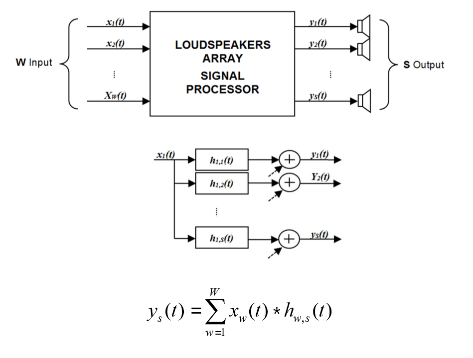
Basically W is Ambisonics, S is what the speaker actually plays back. The next step is the response of the measured environment, which is represented by MIMOIR.

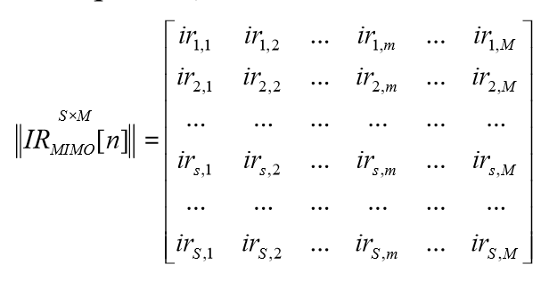
Note that it has as many rows as the number of speakers, and as many columns as the number of microphones.

Then we need to decode the signals from the microphone array to an ambisonics signal, which is an A-format to B-format conversion.

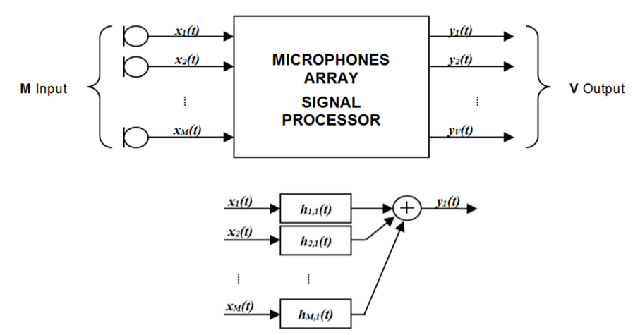
Convolving these three matrixes together we obtain a workflow that goes from a First Order Ambisonics with arbitrary directivity to a Third Order Ambisonics that already accounts for the measured environment and for the equipment employed in the measurement.

Time alignment

While the original MIMO workflow relies on keeping source and receiver perfectly in sync, we cannot do that, due to the need of having a portable system that does not rely on mains electricity. We don't currently have an amplifier capable of powering the loudspeaker system while being controlled by the computer, that doesn't also require more power than we can provide in the field.

In order to re-establish this syncronicity, we rely on the fact that channel 1 of the speaker and of the microphone face each other during the first sweep, and that they are the only pair directly looking at each other. Therefore, the first sweep of the first channel will be the loudest.

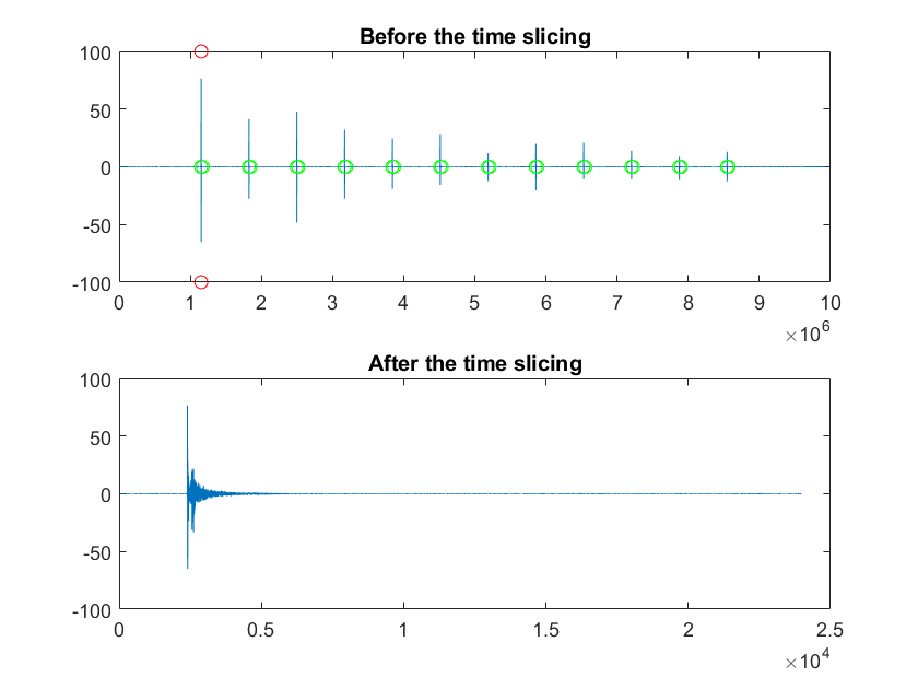
We take the first channel of the file recorded in the field (RecSweep), we convolve it all with the inverse sweep and we obtain one channel of IRs.
To form the MIMOIR we need to put these IRs in a matrix, so we need to slot them in the right column, but the offset between the beginning of the recording and the first sweep changes every time, while the time difference between the first sweep and all the other IRs is fixed. This also allows us to reconstruct the time relationship between the sound source and the receiver, which is necessary for Chiesi's more advanced analysis scripts, like the ray tracing one. We haven't actually used them yet, because they require a 3D model of the environment. Anyway, once we have this sequence of IRs we just take the maximum peak, which we know comes from the first sweep:

[maxPeak, maxIndex] = max(convRes);
and we use maxIndex to trim around the IR. The script is set up to produce a IR of N samples, where N is the sampling rate times the duration in seconds, currently 48000*0.5. So we set the beginning of the IR at 0.1*N sample before the matrix, and the end of the IR at an offset of N samples from that. We also keep into account the silence between the sweeps, which is stored in the variable DeltaSamples, so that we can find the beginning of all the other IRs, and we just apply the timing information from the first channel to all the others

Ambisonics workflow

We want to go from an Ambisonics input to an Ambisonics rendering, which can then be played back using headphones or a loudspeaker array. In order to obtain a suitable convolution matrix we need to perform a two-sided convolution between the microphone filter matrix, the MIMOIR matrix and the loudspeaker beamforming matrix.

This is done with Chiesi's oa_matrix_convconv function:

AMBI3IR = oa_matrix_convconv(hSpk,MIMOIR,hZylia);
Where hSpk is the speaker beamforming matrix and hZylia is the speaker beamforming matrix.

Speech Transmission Index

For a brief explanation of what STI is, and how it's classified, see the Wikipedia article.

First of all, it was necessary to calibrate our whole signal chain. We brought all the equipment to a semi-anechoic room in Terrassa, and we reproduced a series of test signals (exponential sine sweeps, pink noise and the STI-equalized noise), compraing the results obtained recording with the Zylia and with a Brüel&Kjaer sound level meter. We found that the Zylia maxes out at 130dB, exactly as advertised. Knowing the gain of the loudspeaker and the gain of the Zylia we can reconstruct the actual level of the whole chain. This allows us to simulate the reproduction of the STI test signal in the environments where we performed our MIMO measurements.

Here's how to compute the STI using MIMO impulse responses and the Aurora plugins. We need a STI-Signal, which corresponds to the IEC-equalized pink noise that is supposed to be used as a test signal, a STI-Noise, which is the background noise on-site, and a STI-IR, which is the convolution of our MIMOIR with the Zylia beamforming matrix.
We take the W channel of a Zylia recording, of which we know the equivalent level measured with a sound level meter. We open Aurora's STI module, we set the full scale value to 130.33dB minus the Zylia gain, and we press Compute Octave Band Spectrum. We should obtain the same A-weighed level as what was shown by the sound level meter.

As a note, it's better to keep the Zylia gain to 0 in most cases, as it's just a digital gain. In the Siberia fieldwork campaign we usually kept the gain at 30dB, so the fullscale value would be 100dB. To obtain our STI-Signal we must convolve the equalized pink noise, New-STI-step2-PinkNoise-Gain=-26dB_24bit.wav, with the convolution of MIMOIR and the Zylia's beamforming matrix. We recreate what we would have obtained by just playing the equalized pink noise in situ.

In order to obtain STI-Noise we take the silence between our sweeps, of known duration, with one second of margin on each side, and with a 256 samples crossface. We convolve this with the Zylia beamforming matrix and we only keep the W channel.

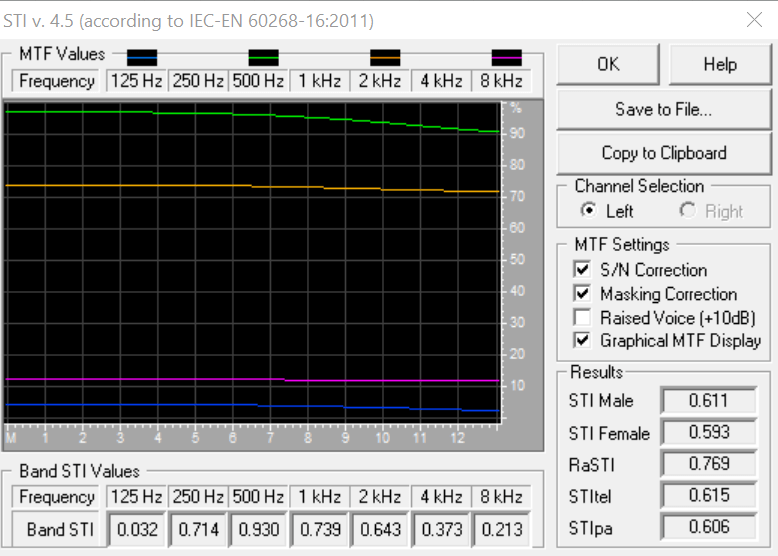
In short, the procedure for calculating the Speech Transmission Index: in an Aurora-compatible DAW we open STI-Noise, then we open the STI module, we set the full scale level based on the Zylia gain, and we click Compute Octave Band Spectrum. Then we click Store as Noise. We repeat this for STI-Signal, but of course clicking Store as Signal. Then we open STI-IR, we open the STI module, and we click on Compute STI. In order to obtain a standard-compliant result, use the settings shown in this screenshot.

Calculate the Strength parameter

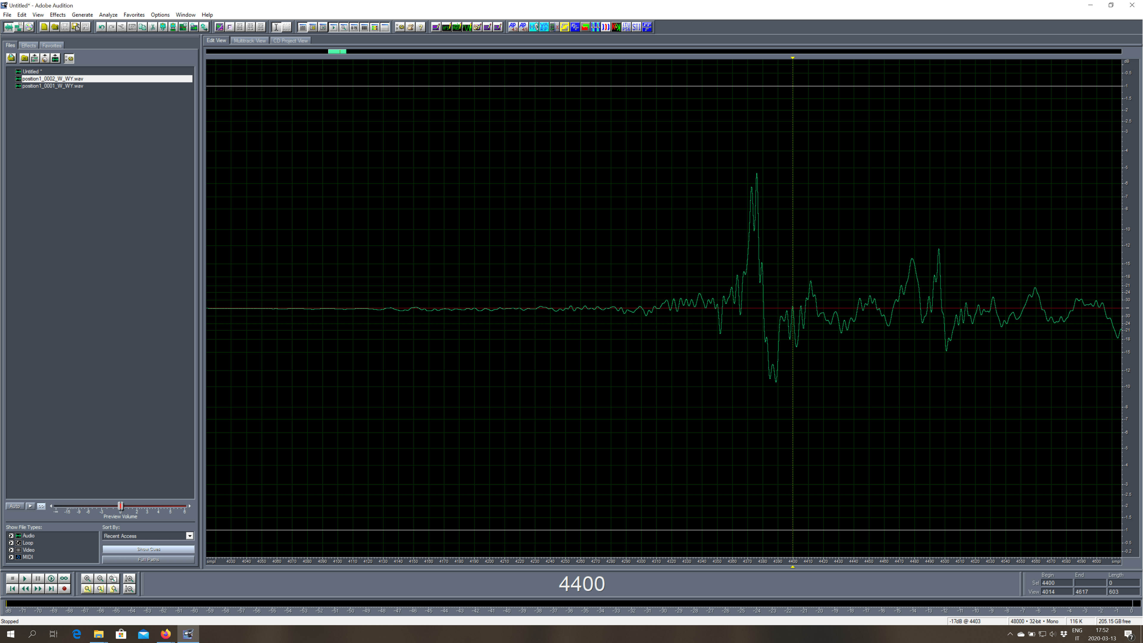
We take the W_WY output file, and we work on the first channel (W). We have to approximate an anechoic IR, so we silence the file from a zero-crossing just before the first reflection, all the way to the end of the file. The difficulty in doing this depends on the specific Impulse Response, here is an example.

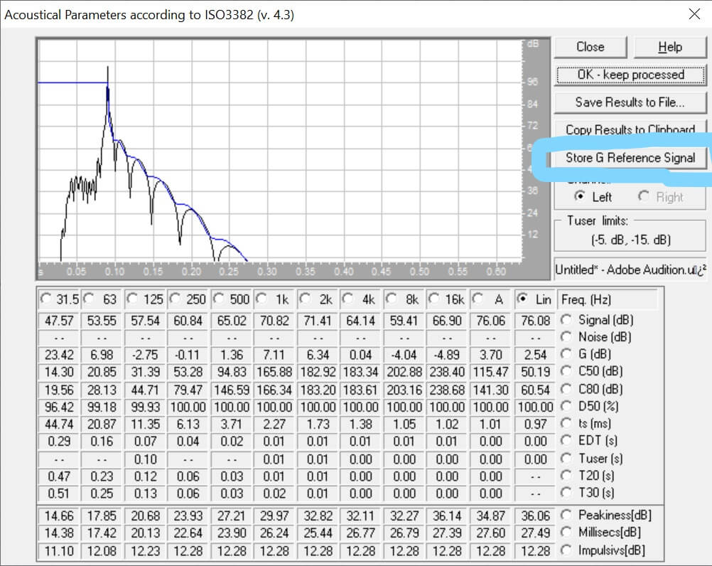
Once we have silenced the reverberant part of the IR we select all, open the Acoustical Parameters module, and we click on Store G Reference Signal, like in the screenshot below.

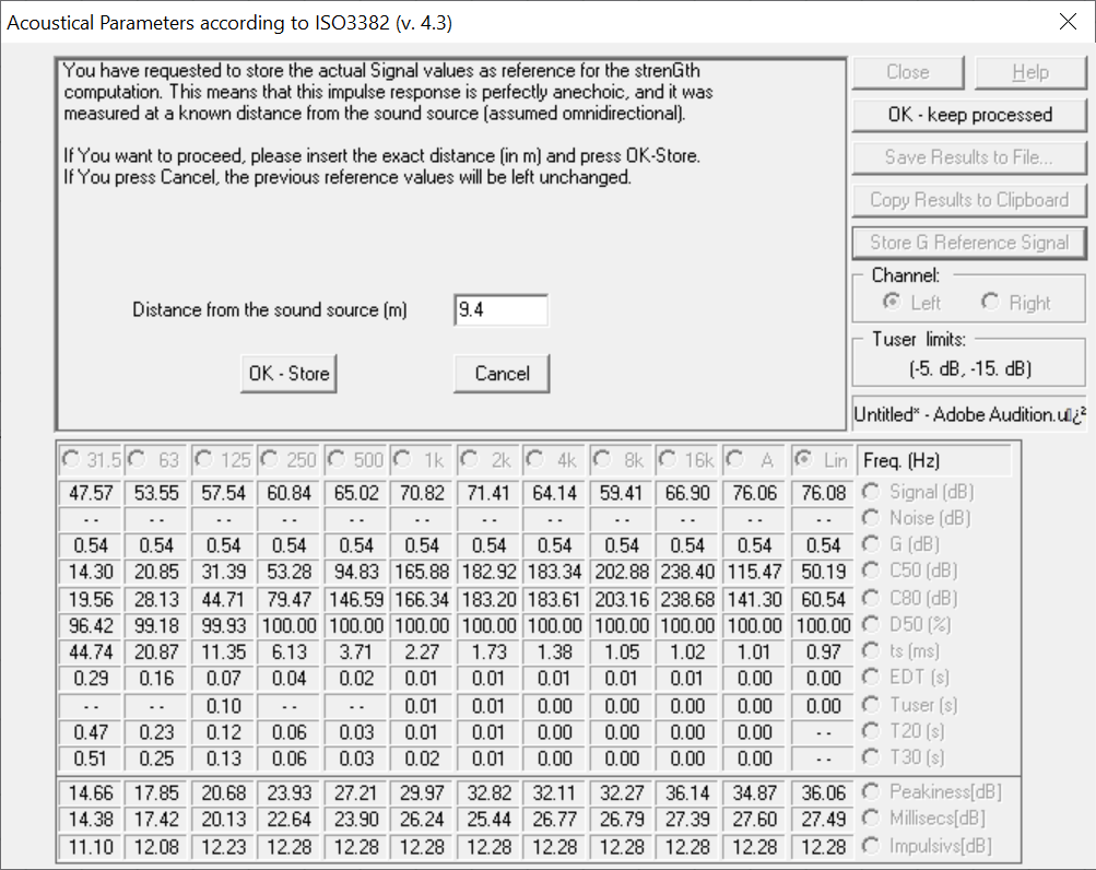
The next step is setting the distance between source and receiver.

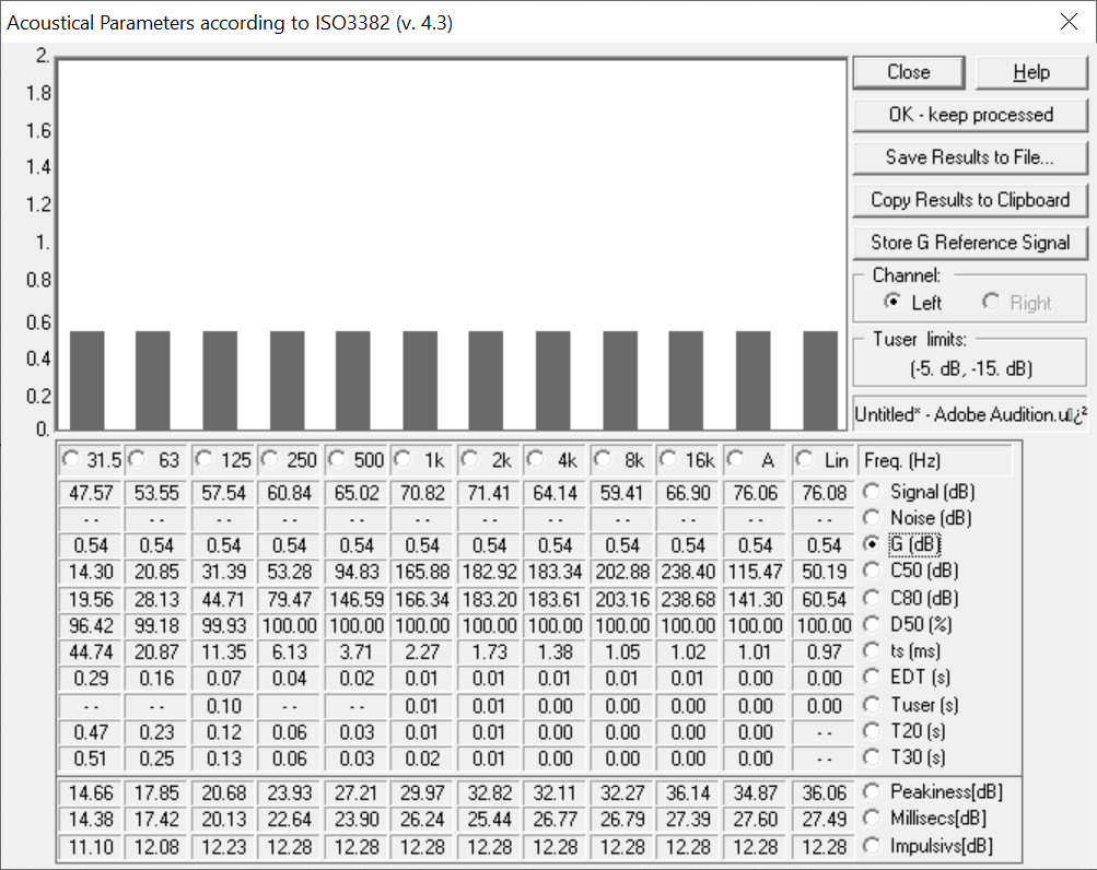
Then we go back to the original IR (complete with the reverberation), and we just calculate the Strength.

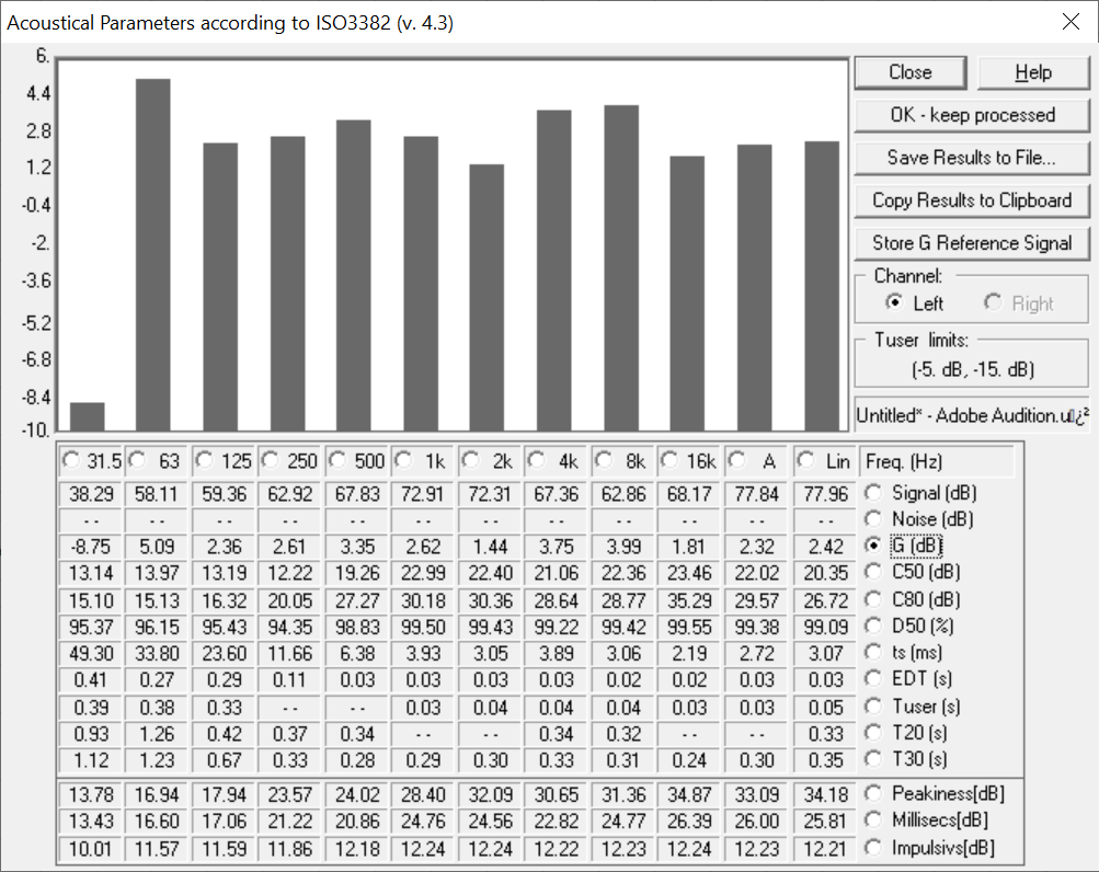
Having multiple positions of a same site we can can calibrate just once, choosing the cleanest IR.

Acoustical Parameters

In November 2020 my father managed to make his Acoustical Parameters module, out of the Aurora plugins, as a standalone command-line utility.

It automatically calculates the ISO 3382 acoustical parameters, taking a WAV file as input. Three versions exist: AcouPar_bin for binaural IRs, AcouPar_omni for omnidirectional IRs and AcouPar_pu for WY Ambix IRs, which is what we have. It was therefore quite straightforward to call this script on every IR batch-processed by the MIMO script, obtaining a complete table of all the measurements done in a fieldwork campaign. This table is stored in the file acoupar_pu.txt, situated in the root folder of the MIMO script, and it can be read as an Excel file.

In the normal processing of acoustical parameters using Aurora there are some modifiers that should be handled by the user, and they are not currently made available in the command-line version. In particular we are not handling the full-scale values and the Strength calibration. So the Strength values produced by this script are not yet correct. However, they are all generated with exactly the same methodology, so they can still be used for comparing sites relatively to each other.

Further Developments

These are the next steps we are planning for this script (and not for the workflow more genrally):

• Creating an angle-dependent STI parameter, called STI(θ)
• Reimplement the convolution, which is by far the worst performance bottleneck, in C