MIMO acoustical measurements: how we got here
Table of contents
- Brief history of acoustical measurements
- Impulse Responses
- The state of the art of acoustical measurements
- Ambisonics
- The first MIMO loudspeaker array
- The current MIMO loudspeaker array
- The measuring procedure
- Further development
- Processing the measurements
This is an adaptation of a post written for the Artsoundscapes blog. The idea is to expand it and make it more interactive and hypertextual, but for now (2020/05/30) this is v1.
By mid-June 2020 I should have embedded sound samples, and examples of the visual mapping of reflections. By the end of June the whole MIMO software pipeline should be ready, capable of going from a measured IR to acoustical parameters, all in a Matlab script.
For the paper that introduced the MIMO technique see Measuring Spatial MIMO Impulse Responses in Rooms Employing Spherical Transducer Arrays, by Angelo Farina and Lorenzo Chiesi, presented at the AES Conference onSound Field Control2016 July 18–20, Guildford,UK.
Brief history of acoustical measurements
The field of acoustics was first formalized at the end of the nineteenth century by American physicist Wallace Clement Sabine (Harvard University), and his research on what characterises the sound of a room. As a result of his work, he introduced the concept of Reverberation Time (T60 or RT60) which is the time it takes for sound energy to decay a million times (-60 dB) from the interruption of sound itself in a confined environment. In practice, it quantifies the duration of the "sound tail" as we perceive it "by ear" (for example, when we clap our hands in a room). It is measured in seconds and, therefore, allows us to evaluate how long it takes before a sound is extinguished in a room. This concept is still in use and it is one of the main measures used in acoustics today.
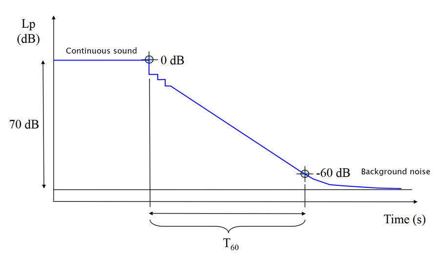
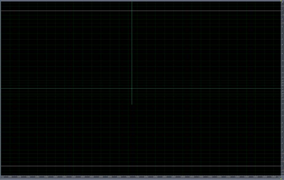
Sabines methodology consisted in producing a continuous loud sound, stopping it, and measuring the time it took for the reverberation to become inaudible. The discrete steps in Figure 1 represent the individual reflections, which act as sound sources that become inactive one by one, as the sound completes its path from source to receiver.
As
the sound source is turned off, the microphone detects no change until the
sound has travelled the direct path between the source and the microphone. This
is the first horizontal bit of the graph, labelled as Continuous sound. When
the direct sound ceases, we can see a first drop in the sound level. As the sound
can arrive to the source after any number of reflections, we will see a long sequence
of level drops, ordered by the length of the path taken by the sound, called
the reverberant tail, until only the background noise is left.
Today, however, this technique has been almost completely abandoned in favour of
methods based on the measurement of the Impulse Response (IR) of the
environment under examination.
Impulse Responses
The Impulse Response, at its most basic, is the response of a system to a stimulus. With a few basic assumptions, we can use the impulse response to determine the response of the measured system to any other stimulus.
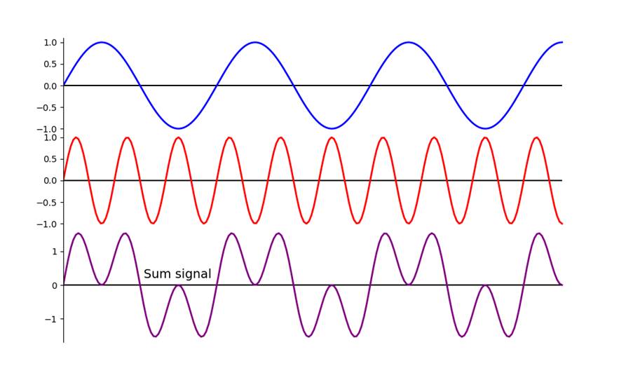
We need the system to be linear and time-invariant. A linear system is one for which the superposition principle applies. This means that the output obtained from inputs A and B equals the output obtained from the arithmetic sum of the individual inputs. In mathematical terms: y(A)+y(B)=y(A+B)
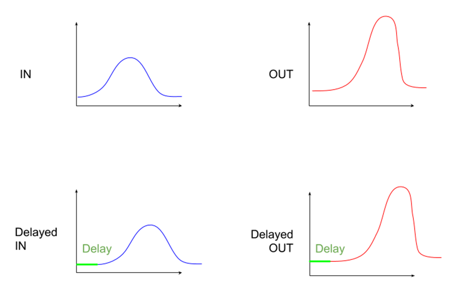
A time-invariant system is one that gives the same output if given the same input at different times. In mathematical terms:
y(t)=T[x(t)]
y(t-t0)=T[x(t-t0)]
In graphical terms:
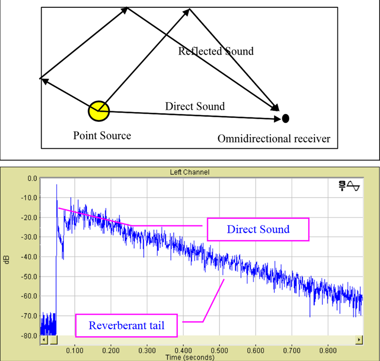
So, assuming we can model the room that we are measuring as a linear time-invariant system (which is often not entirely the case, for example temperature changes can affect the acoustics), we can use impulse responses for our measurements. Figure 4 depicts the basic setup.
The state of the art of acoustical measurements
In acoustics, the traditional method for performing impulse response measurements is very literal: we produce a loud bang and we record what happens.
Both the sound source and the microphone used to record it need to be omnidirectional, meaning that the sound radiates equally in every direction from the source, and that the microphone is equally sensitive to incoming sounds from every direction. Figure 5 depicts some of the most common microphone directivity patterns.
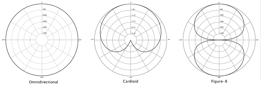
Omnidirectional microphones are widely available, and common sound sources include balloons, guns and firecrackers. These are fun to use, but they cannot be used in every location, for example for travel-related reasons (airport security strongly dislikes gunpowder residue in your hand luggage). There are also restrictions because of conservation reasons, as some environments are too fragile for explosions, while others are so loud (in terms of always present background noise) that it is difficult to achieve a usable signal to noise ratio (refer back to Figure 1). Balloons are still a very good backup, last summer we brought with us more than 800 of them to the Artsoundscapes projects fieldwork in Siberia, just in case something went wrong with our loudspeaker!
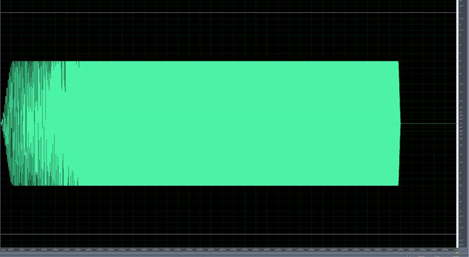
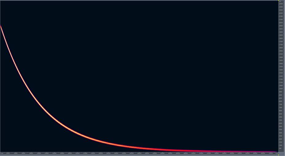
In the past years, in order to overcome some of these problems (travel restrictions, signal-to-noise ratio and conservation concerns) new methodologies for the measurement of impulse responses based on the use of loudspeakers have been developed. The use of signals such as MLS (Maximum Length Sequence) at first and then LSS (Linear Sine Sweep) and ESS (Exponential Sine Sweep) are common. LSS and ESS are mathematically complex signals, but they have some extremely useful characteristics. By convolving the acoustic response of an environment with the inverse (Figure 8, Figure 9) of the sine sweep that we played in that environment (Figure 6, Figure 7), it is possible to obtain an impulse response with a great signal to noise ratio and cleansed of all the non-linearities of the audio system used. Non-linearities are the outputs of the system that dont conform to the linear model explained above: basically, in our case, they are distortions in the signal chain caused either by the amplifier or by the speaker driver themselves.
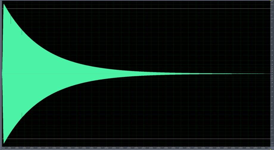
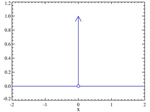
If we convolve the test signal with its inverse, a Dirac delta is obtained (Figure 10). The Dirac delta is a theoretical signal (Figure 11 with some pretty interesting characteristics, but to put it simply it is a sound file in which all samples are 0, and just one sample is 1.
However, if one of our measurements is convolved with the inverse sweep, an impulse response is obtained, one with all the non-linearities on the left (before, in time), the direct sound looks just like a Dirac delta, and all the subsequent reverberations are smaller peaks on the right.

Ambisonics
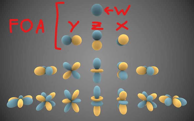
At the same time that the methods to measure impulse responses have evolved, microphones have also developed. They are now able to capture more accurate spatial information. This started with the work of mathematician Michael Gerzon in the 1970s, and the technique has become popular in the last decade thanks to VR. Some really good work has already been done using omnidirectional sound sources and Ambisonics microphones: arrays of microphones that encode the spatial information of sound using spherical harmonics, capturing both the pressure and the particle velocity of the incoming sound. This allows us to visually map where the sound is arriving from, and for listening to the recordings using headphones or loudspeaker arrays, perceiving the directionality of sound. Regarding microphone arrays, in particular, the evolution has been from the four faces of a tetrahedron (i.e. Soundfield Mic) to spherical arrays, such as the Eigenmike or the Zylia that we are using in the Artsoundscapes project.
The first MIMO loudspeaker array
Just a few years ago, Professor Angelo Farina (University of Parma) and Lorenzo Chiesi innovated the field of acoustical measurements with the development of a sound source of variable directivity. A sphere of loudspeakers - each with its own amplifier - was assembled and, using the same mathematics as Ambisonics, it became possible to have the sound source radiating with arbitrary directivity. With this technique it is possible to have an omnidirectional source, or a source with the directivity of the human voice, or of a musical instrument, all with the same hardware.
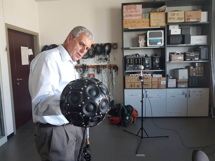
The original MIMO array was a sphere with 32 loudspeakers, each connected to a separately stored amplifier. The amplifiers weighed several kilograms, they required mains power, and the cables connected to the speakers, even if they were just 1m long, were very thick and very heavy, just because of their sheer number.
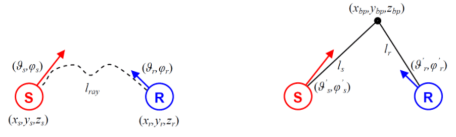
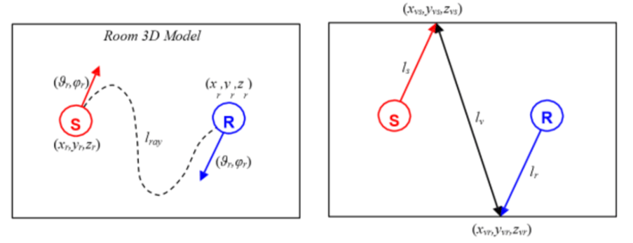
With this new source system and a microphone array, it is possible to execute MIMO (multiple input, multiple output) impulse response measurements, which allows us to trace the sound path between source and receiver, showing where each reflection occurs.
The current MIMO loudspeaker array
For the Artsoundscapes project we had to accommodate stringent weight and energy requirements.
All the equipment was to be used in the field, away from electricity sources for several days. Furthermore, it had to be brought to remote locations, where wheels are not an option. It was supposed to be shipped on planes, which gave us size and weight limits. It also required a certain amount of mechanical resistance to rough handling, and forced us to think hard about what components can be legally shipped. Lithium batteries had to be taken as hand luggage, for example. Instead of mains, our source of electrical power would be the Voltaic battery pack, which could provide voltages between 5 and 24V.
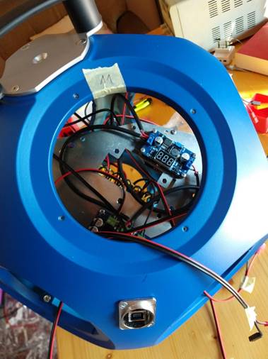
It was decided to switch to a classic loudspeaker shape, the dodecahedron, a solid composed of twelve pentagonal faces, very commonly used for omnidirectional loudspeakers. To further save on both weight and electricity, all the electronic components were put inside the dodecahedron. In theory, this simplified usage in the field, but in practice it forced us to use a larger dodecahedron, which affected the directivity at higher frequencies. This also made it harder to troubleshoot the loudspeaker array if something went wrong.
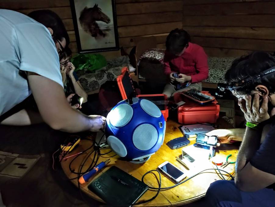
Just one amplifier was used, which meant that just one loudspeaker could be used at a time. This caused the measurements to take slightly longer than if we had used all the loudspeakers simultaneously, but it was not really a problem, as the real bottleneck was the setup process.
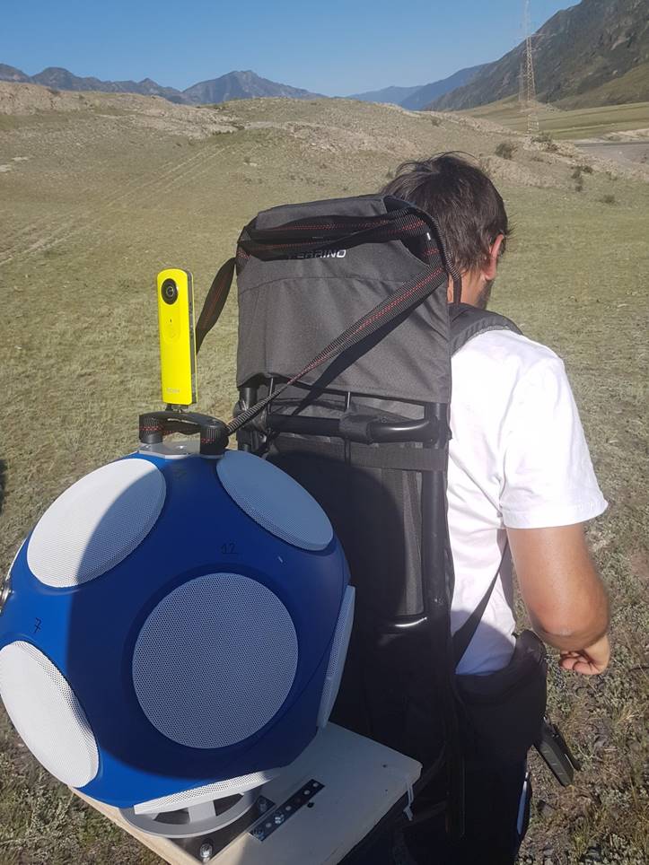
Finally, in order to perform the visual reconstruction of the sound path, it is crucial to acquire panoramic images from the same position and orientation as both the source and the receiver. This is done with Ricoh Theta cameras, which employ standard photographic screws. The mounting system for the loudspeaker had to be designed taking into account the need to slot the loudspeaker on a tripod, to transport it securely both in its carrying case and a special backpack, and to mount a panoramic camera on its top.
At the bottom the loudspeaker had a simple cylindrical mounting point, which allowed for quick slotting over a tripod, without finicky screws or locking mechanisms. This mounting point was also used with the carrying case and with the backpack, making the whole apparatus unable to move during transport. At the top, a modular plate allowed for screwing in a handle, which was itself threaded for photographic screws.
The measuring procedure
In our fieldwork in Siberia the new MIMO array output the same sweep twelve times, each time from a different loudspeaker. In order to do this, it was necessary to build a control system which could effortlessly execute this sequence. A Zoom H2n recorder was used to play back the file containing our test signal on the left channel, and a special series of clicks on the right channel. A Zoom was used instead of a phone because it made it easy to keep a consistent gain. It was connected with a 3.5mm jack to the array, inside which an Arduino board received the right audio channel and counted the clicks, connecting the appropriate speaker to the amplifier using a relay board. In practice the amplifier was always connected, as the relays change which loudspeaker receives the signal on the left channel. The only other cable needed was the power cable, which allowed our Voltaic batteries to provide the 19V we need. These batteries had enough capacity to power our array for several hours, and they could even be recharged with solar panels, providing us with weeks of autonomy. However, the amplifier used tended to distort at the power levels actually employed, which limited our signal to noise ratio.
On the receiver side, we were recording with a Zylia microphone connected to a laptop, as well as with a Brahma: a First-Order Ambisonics microphone mounted on a Zoom H2 recorder, as a backup. On the same tripod as the microphones, another Ricoh Theta was mounted, in order to provide a panoramic image from the point of view of the listener.
Further development
Having completed a month-long expedition in Siberia, as well as several local measurements in Catalonia with the current system, we are already working on ways to improve both its capabilities and its portability. In particular, we would like to switch to a smaller dodecahedron with external electronics. The smaller dimensions would help with the directivity at higher frequencies, as well as with the portability. In addition, the external electronics would make troubleshooting the system easier and allow for easier thermal dispersion. We are also evaluating the possibility of switching to newer multichannel amplifiers, which could allow us to use more than one speaker at a time. This could potentially speed up the measurement procedure and open up new forms of qualitative explorations.
Finally, here's a video of the loudspeaker array in operation, near Ermita de la Pietat, Ulldecona.
Processing the measurement
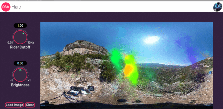
A dedicated Matlab script has been developed. The script itself is available here, and here is an explanation of how the script works