|
1
|
|
|
2
|
|
|
3
|
|
|
4
|
|
|
5
|
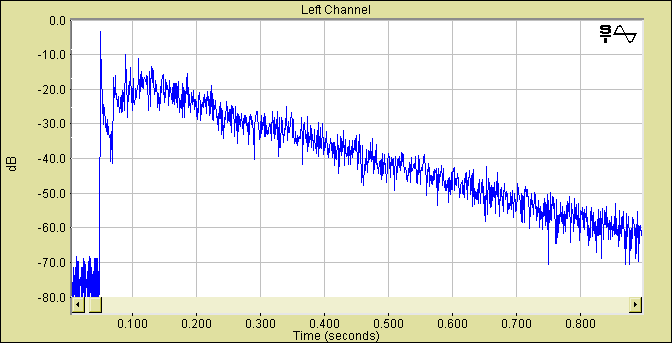
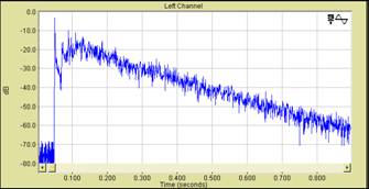
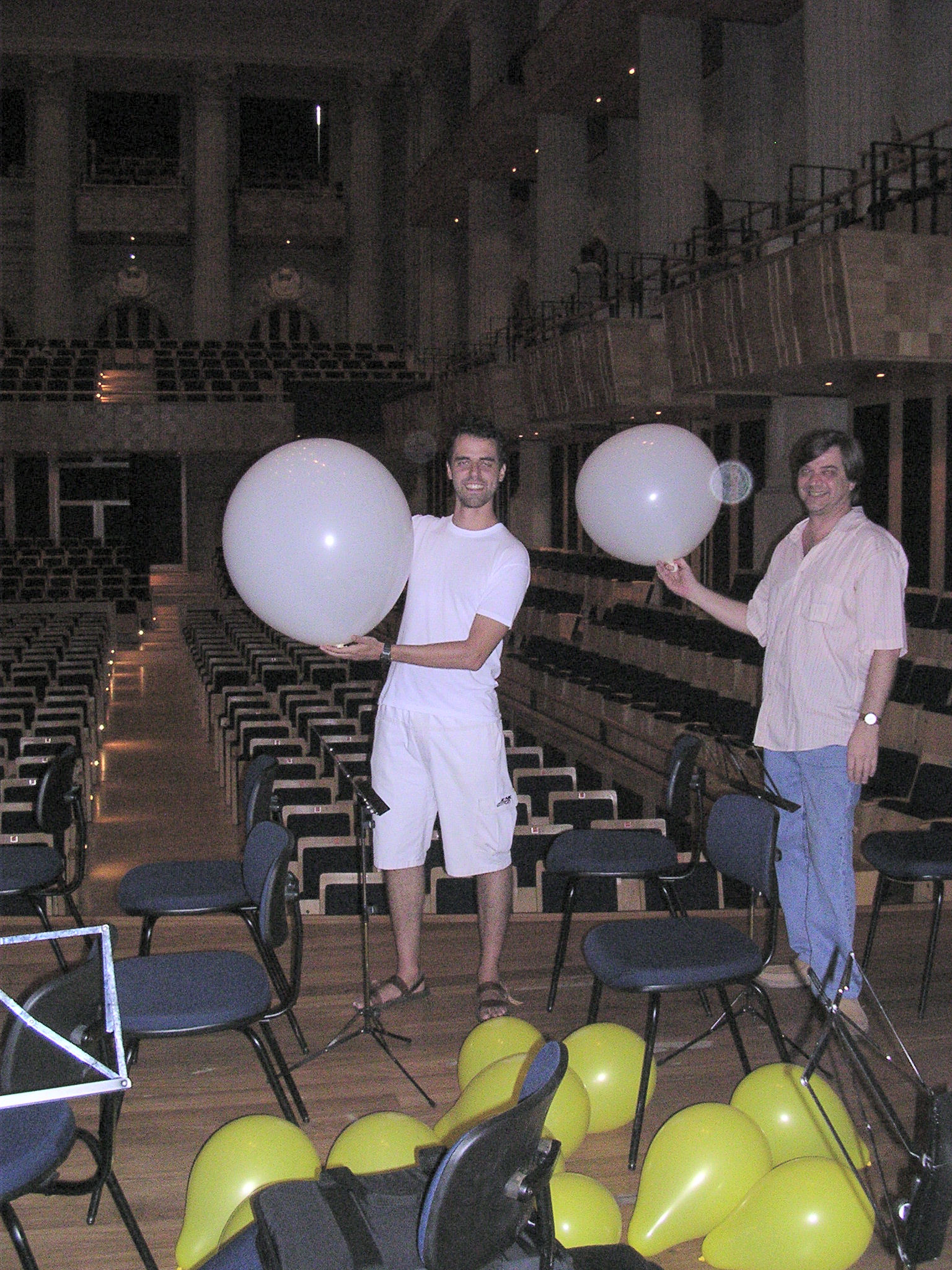
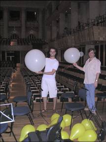
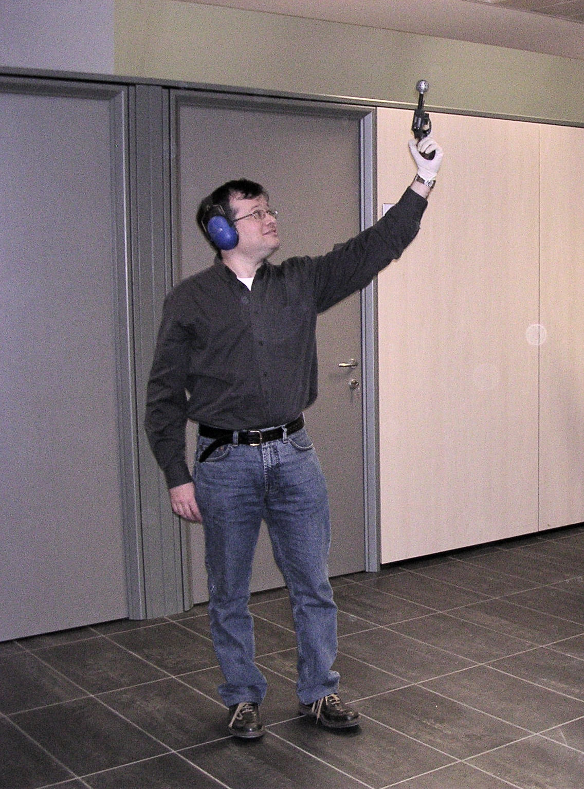
- Pulsive sources: ballons, blank pistol
|
|
6
|
|
|
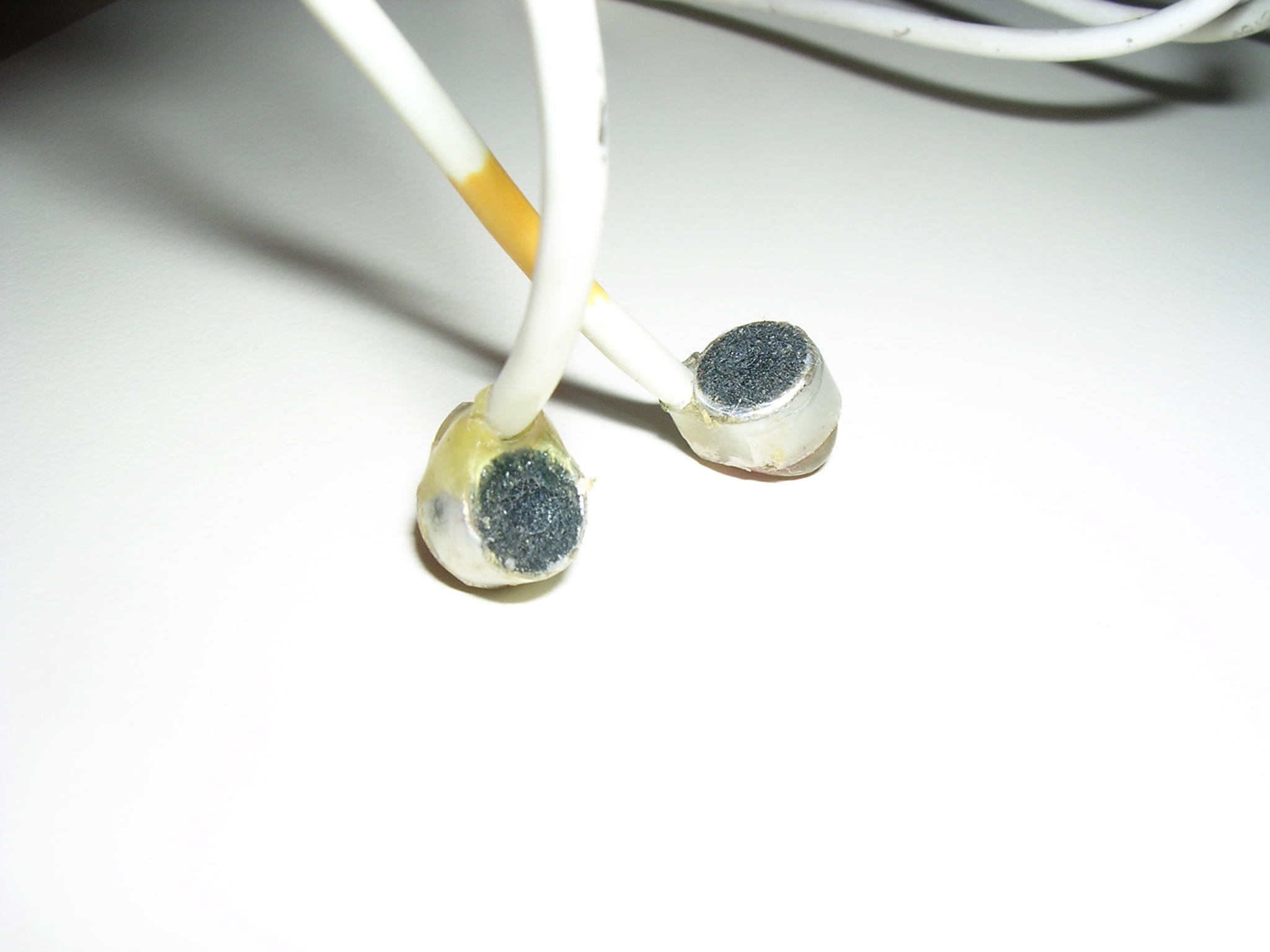
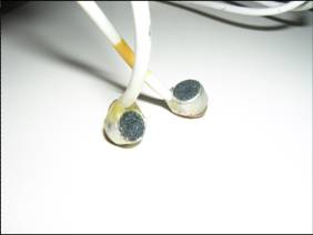
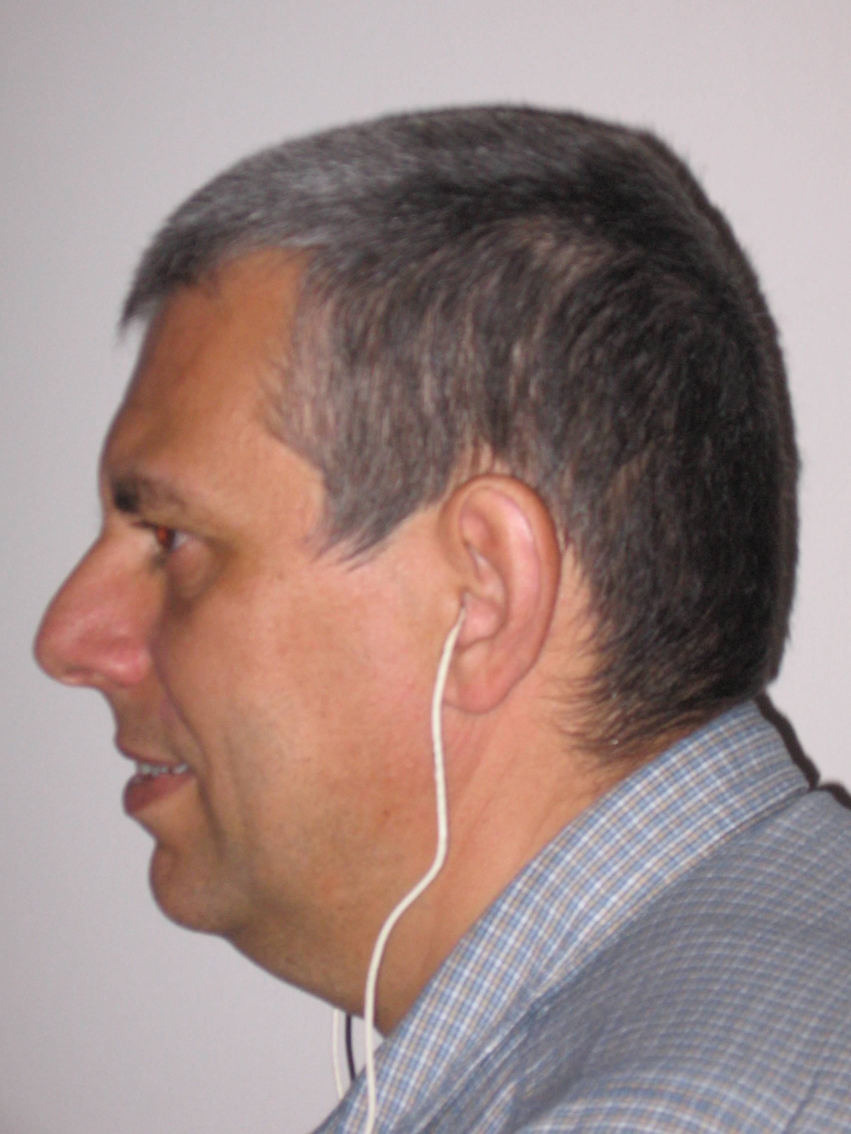
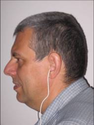
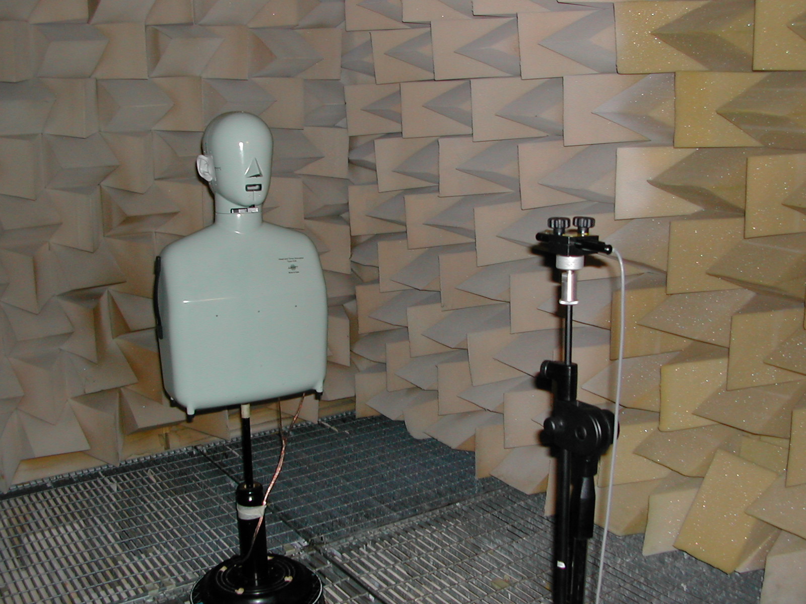
7
|
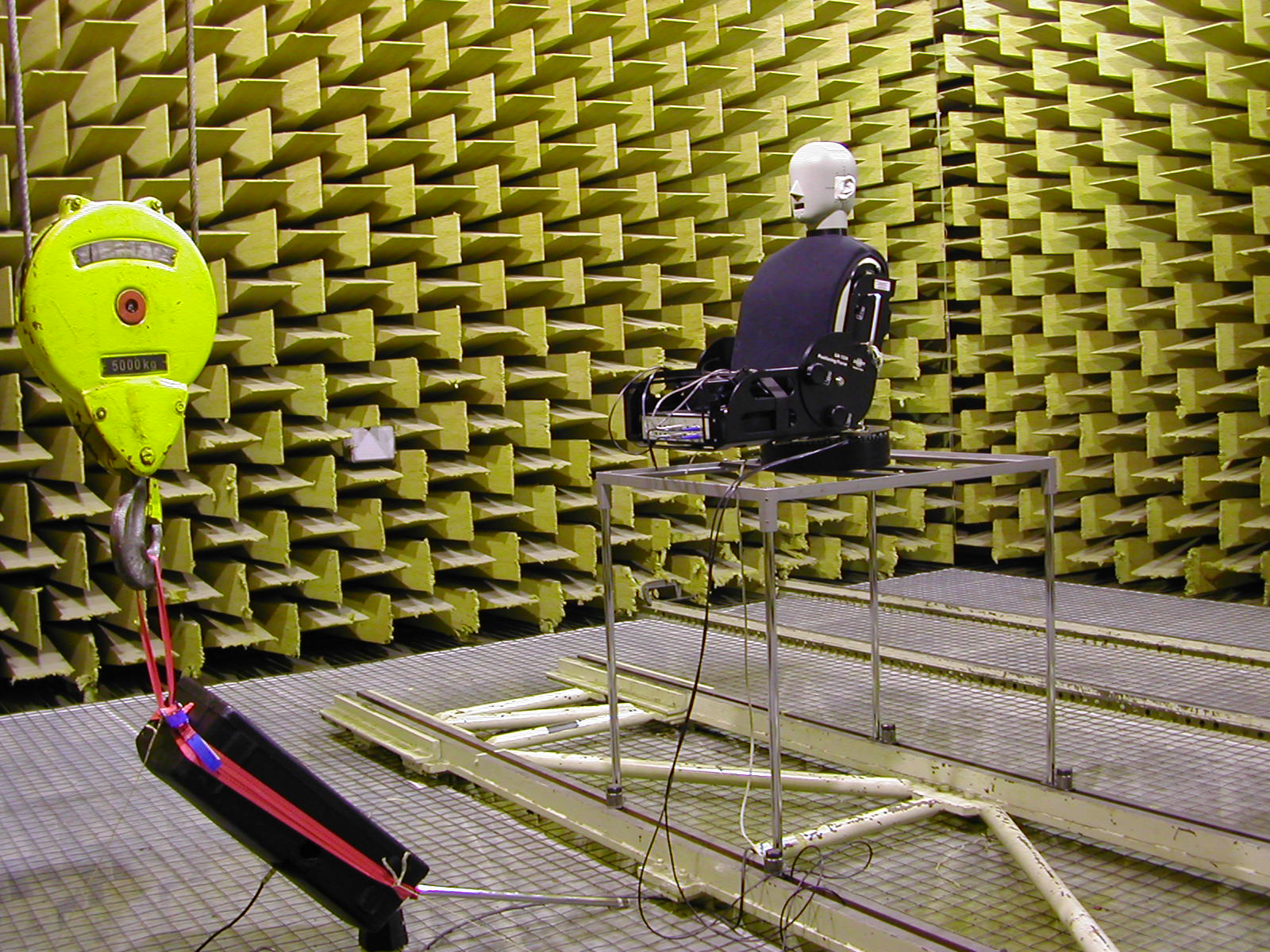
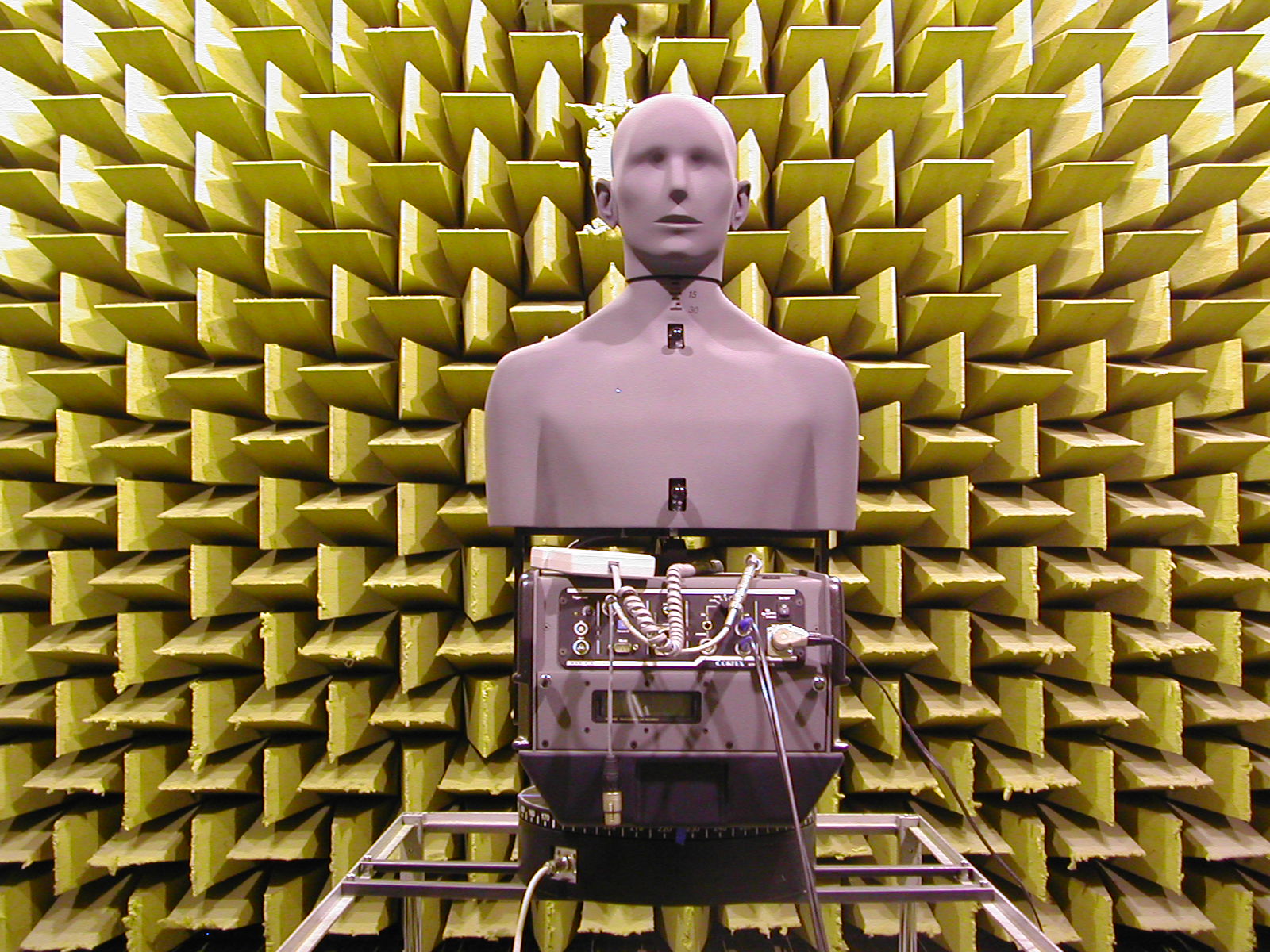
- Cheap electret mikes in the ear ducts
|
|
8
|
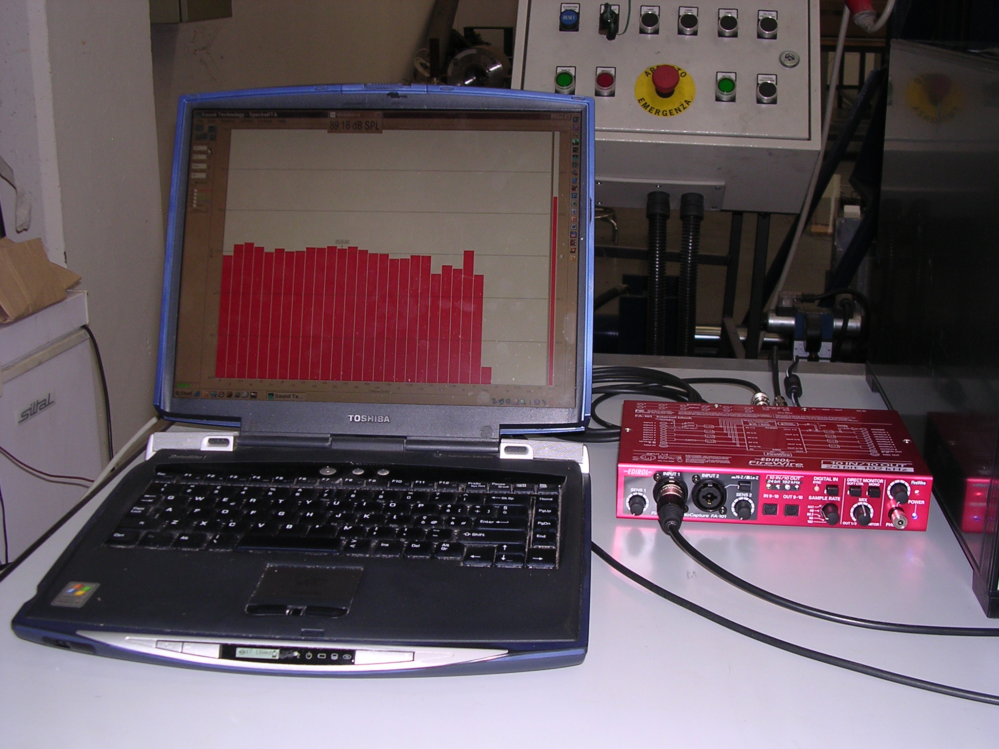
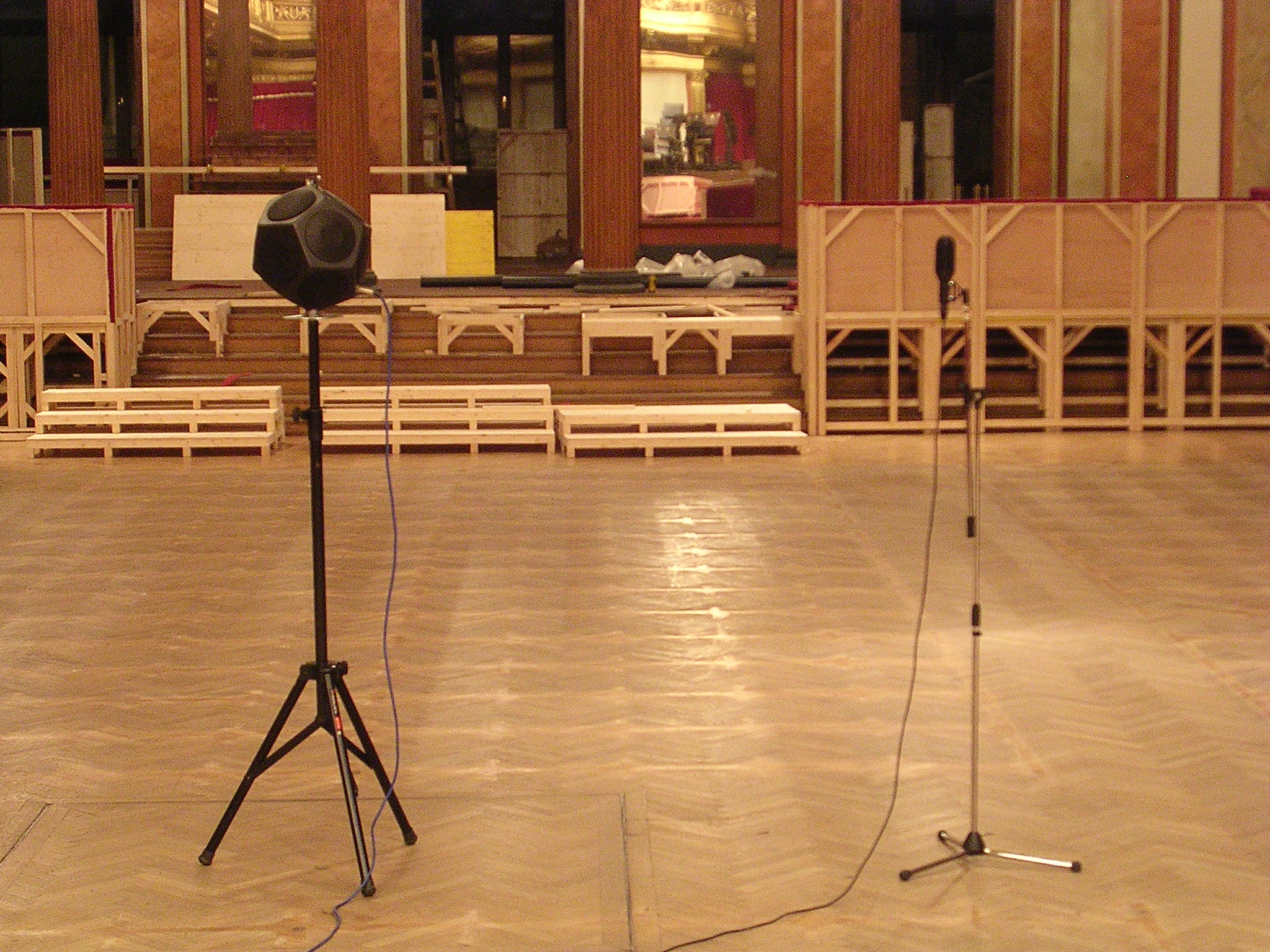
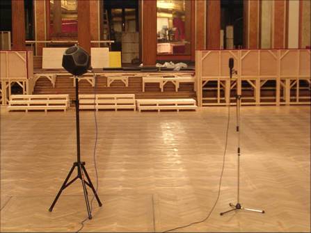
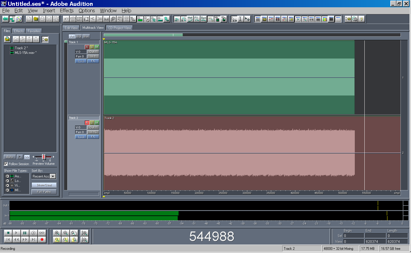
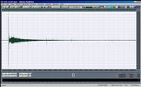
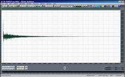
- A loudspeaker is fed with a special test signal x(t), while a microphone
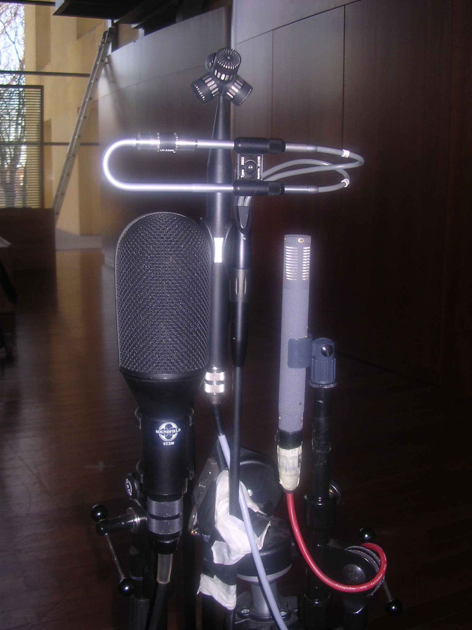
records the room response
- A proper deconvolution technique is required for retrieving the impulse
response h(t) from the recorded signal y(t)
|
|
9
|
- The desidered result is the linear impulse response of the acoustic
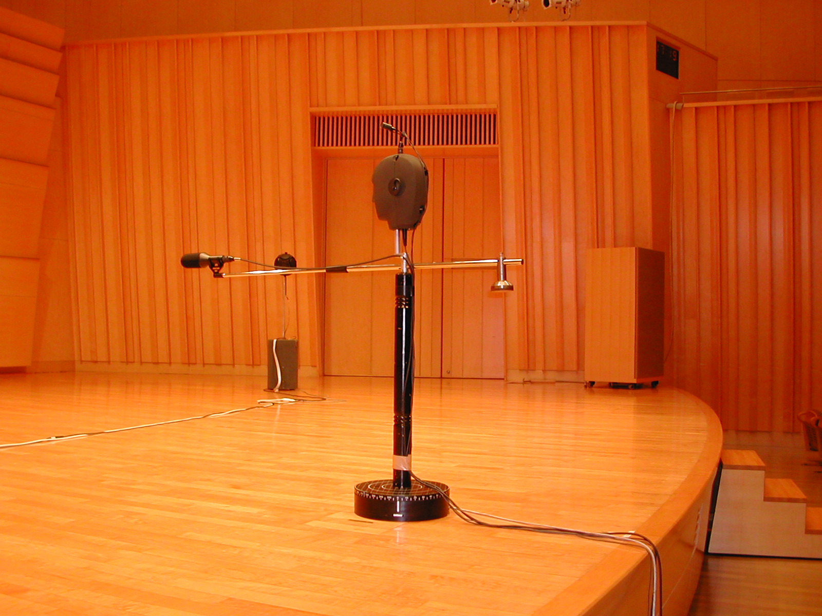
propagation h(t). It can be recovered by knowing the test signal x(t)
and the measured system output y(t).
- It is necessary to exclude the effect of the not-linear part K and of
the background noise n(t).
|
|
10
|
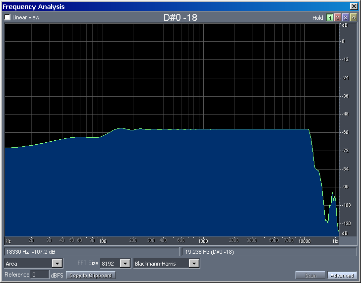
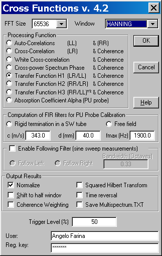
- Different types of test signals have been developed, providing good
immunity to background noise and easy deconvolution of the impulse
response:
- MLS (Maximum Lenght Sequence, pseudo-random white noise)
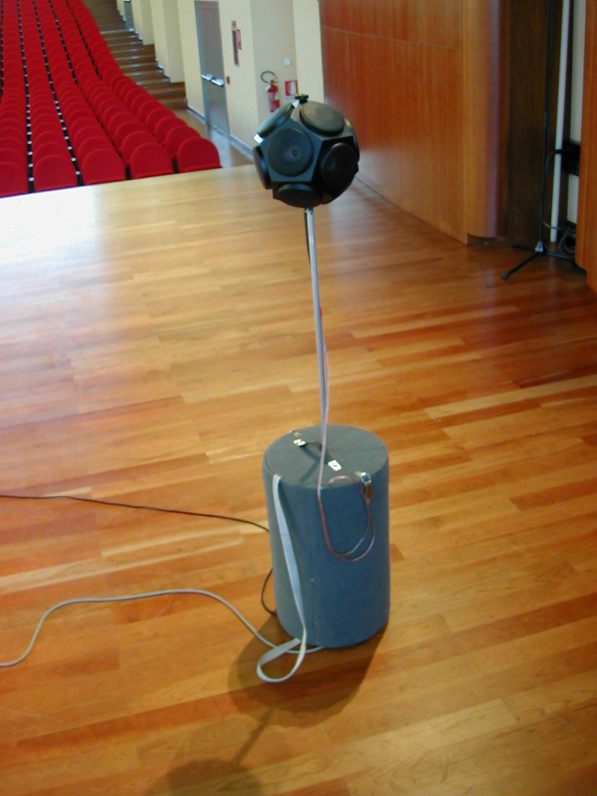
- TDS (Time Delay Spectrometry, which basically is simply a linear sine
sweep, also known in Japan as “stretched pulse” and in Europe as
“chirp”)
- ESS (Exponential Sine Sweep)
- Each of these test signals can be employed with different deconvolution
techniques, resulting in a number of “different” measurement methods
- Due to theoretical and practical considerations, the preference is
nowadays generally oriented for the usage of ESS with not-circular
deconvolution
|
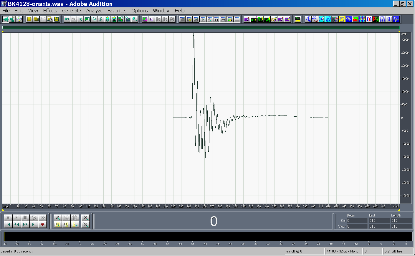
|
11
|
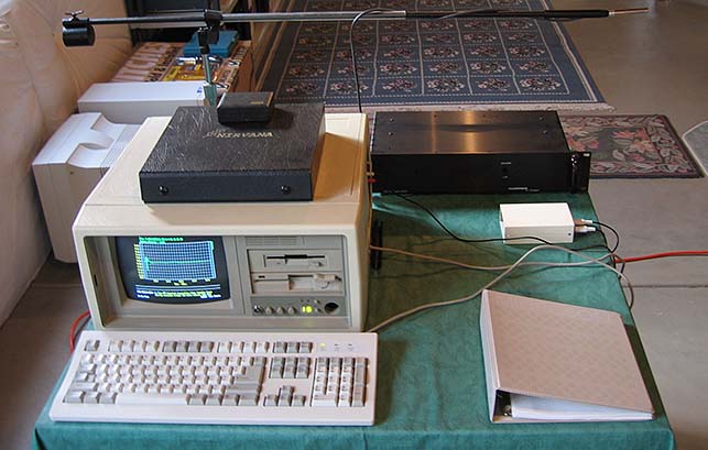
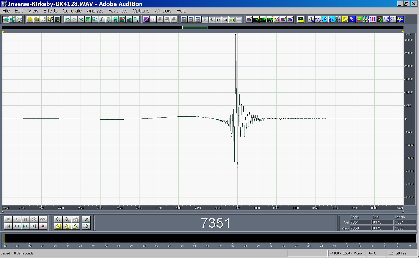
- MLSSA was the first apparatus for measuring impulse responses with MLS
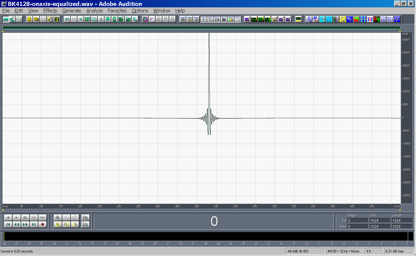
|
|
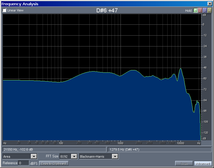
12
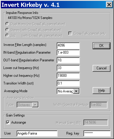
|
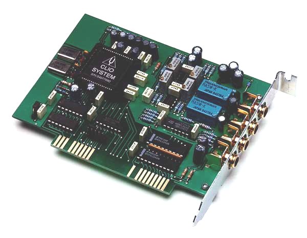
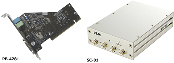
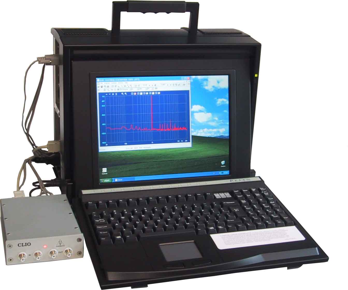
- The Italian-made CLIO system has superseded MLSSA for most
electroacoustics applications (measurement of loudspeakers, quality
control)
|
|
13
|
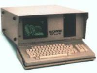
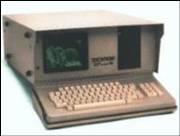
- Techron TEF 10 was the first apparatus for measuring impulse responses
with TDS
- Subsequent versions (TEF 20, TEF 25) also support MLS
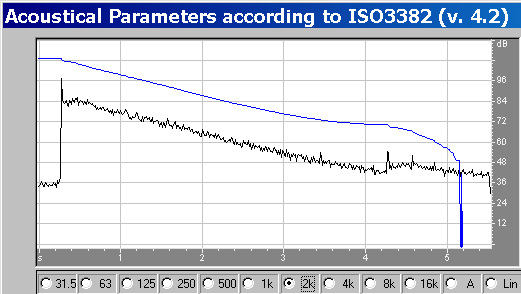
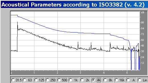
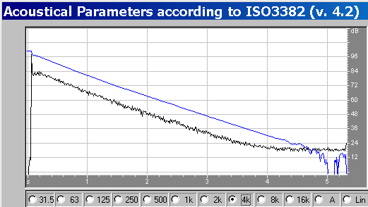
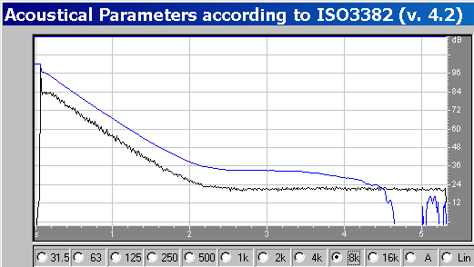
|
|
14
|
|
|
15
|
|
|
16
|
|
|
17
|
|
|
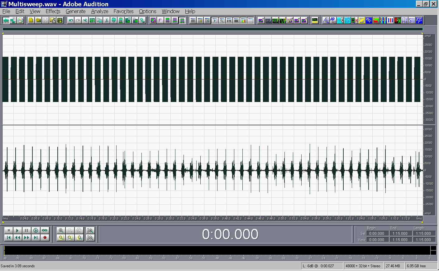
18
|
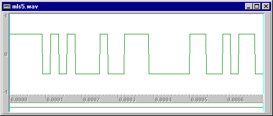
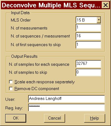
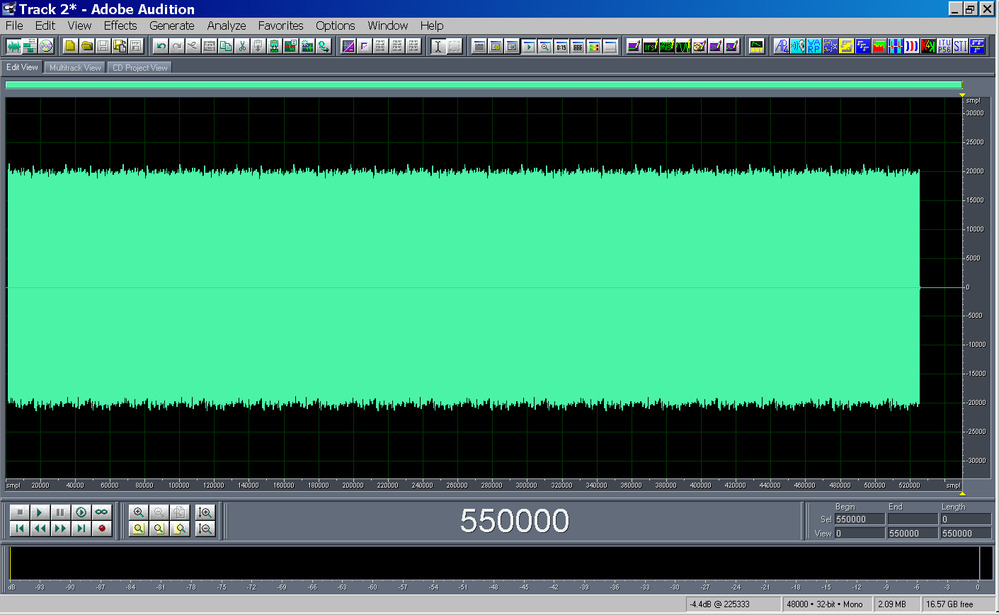
- X(t) is a periodic binary signal obtained with a suitable
shift-register, configured for maximum lenght of the period.
|
|
19
|
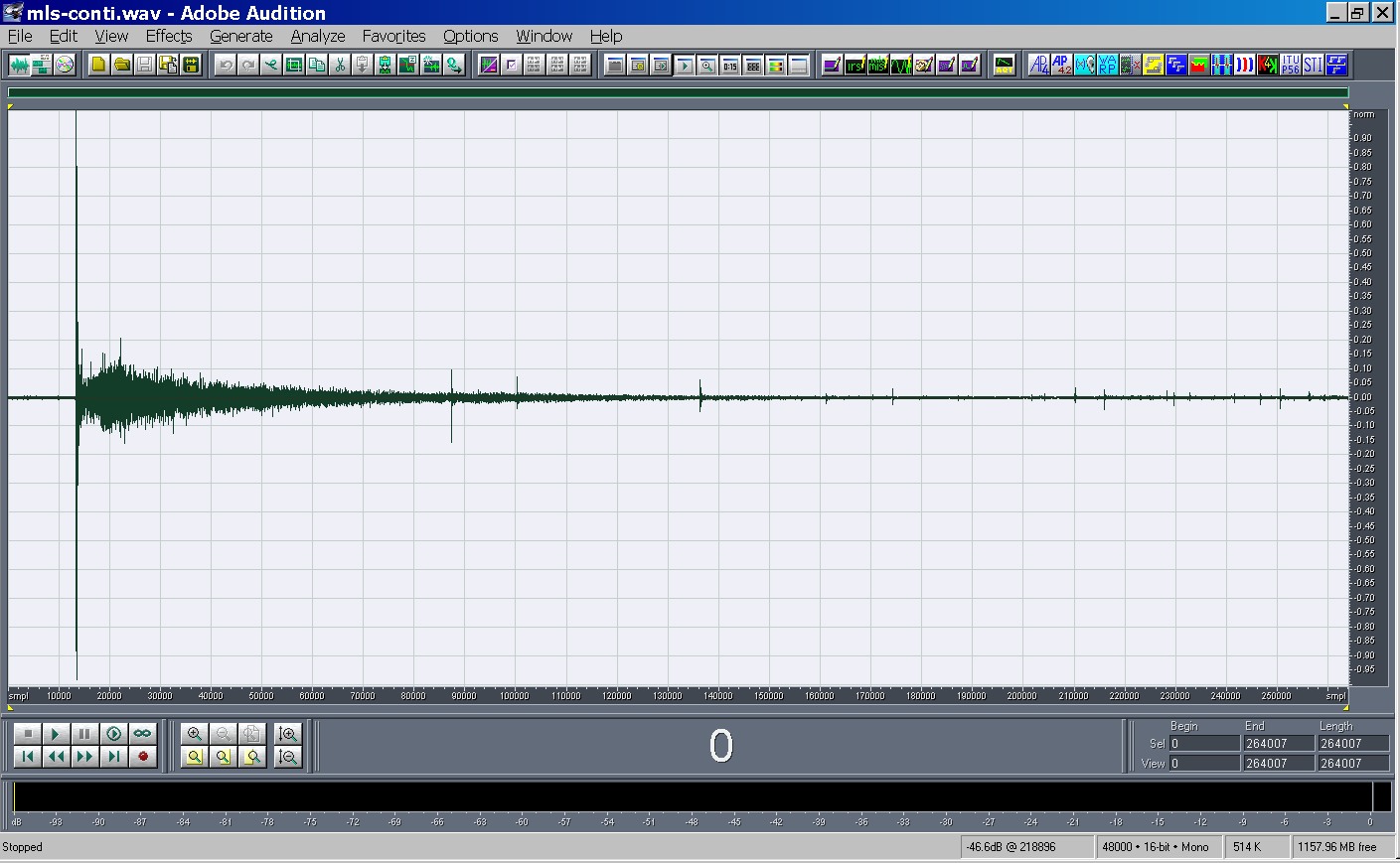
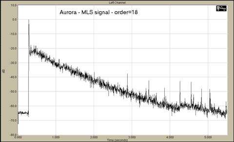
- The re-recorded signal y(i) is cross-correlated with the excitation
signal thanks to a fast Hadamard transform. The result is the required
impulse response h(i), if the system was linear and time-invariant
|
|
20
|
|
|
21
|
|
|
22
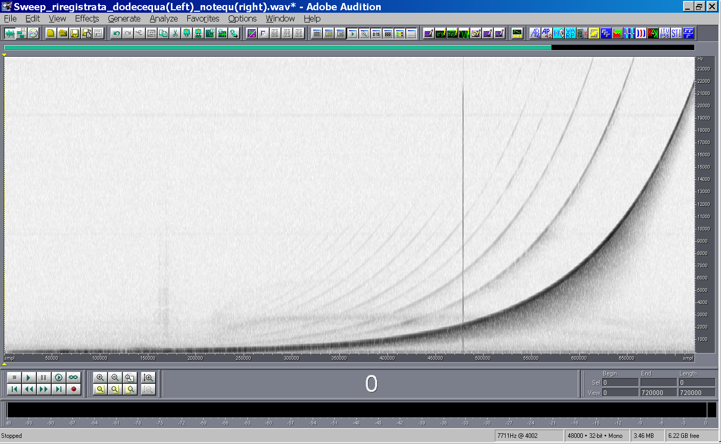
|
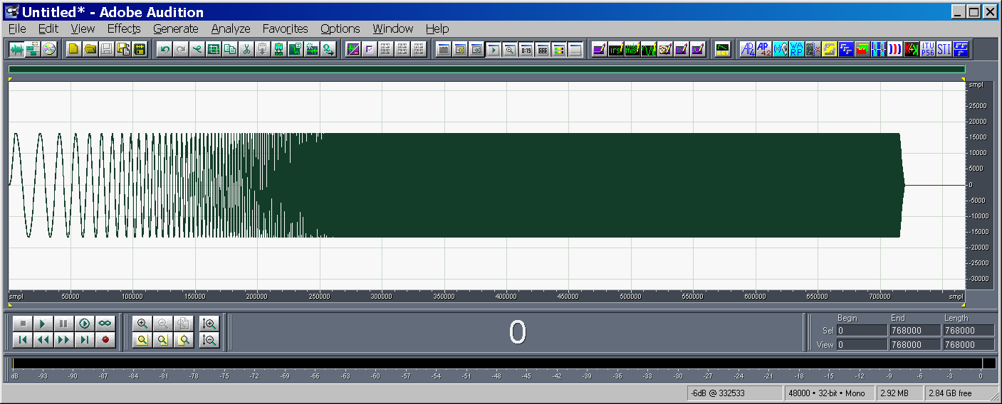
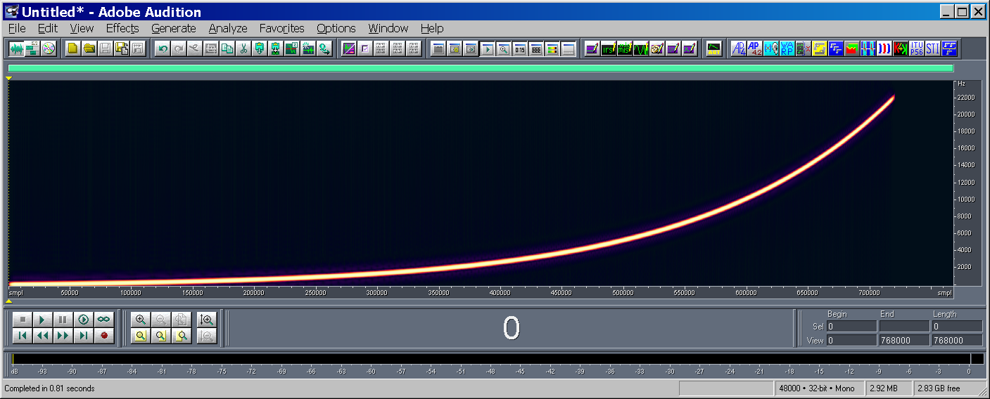
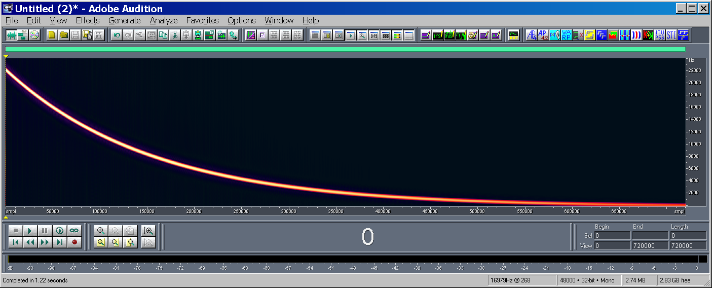
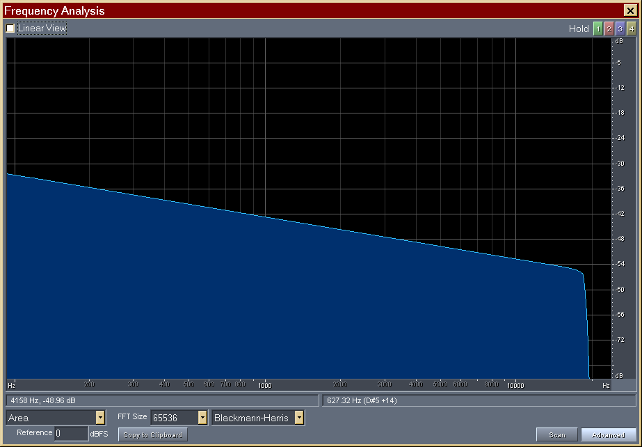
- x(t) is a band-limited sinusoidal
sweep signal, which frequency is varied exponentially with time,
starting at f1 and ending at f2.
|
|
23
|
|
|
24
|
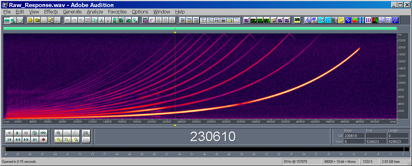
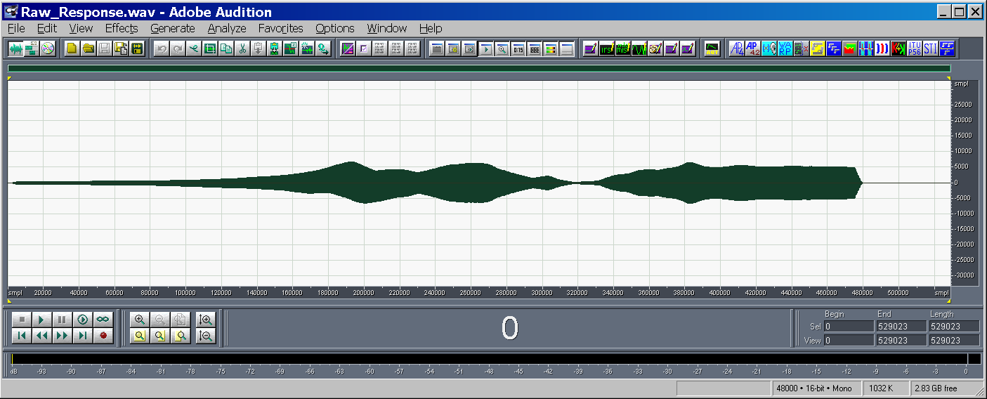
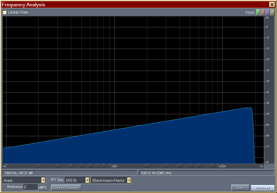
- The not-linear behaviour of the loudspeaker causes many harmonics to
appear
|
|
25
|
- The deconvolution of the IR is obtained convolving the measured signal
y(t) with the inverse filter z(t) [equalized, time-reversed x(t)]
|
|
26
|
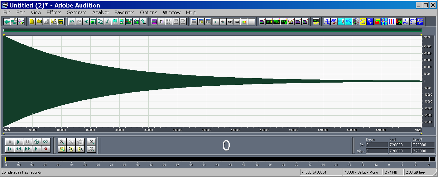
- The “time reversal mirror” technique is employed: the system’s impulse
response is obtained by convolving the measured signal y(t) with the
time-reversal of the test signal x(-t). As the log sine sweep does not
have a “white” spectrum, proper equalization is required
|
|
27
|
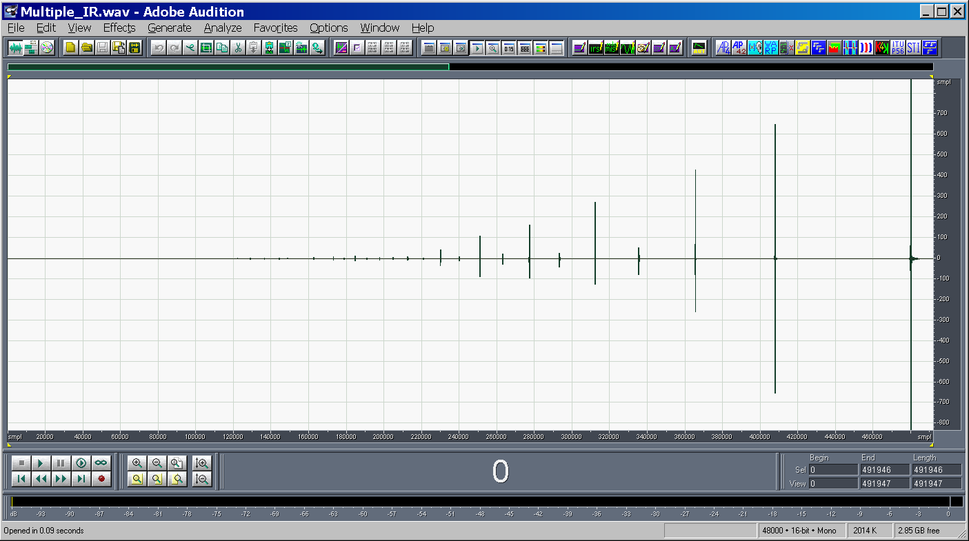
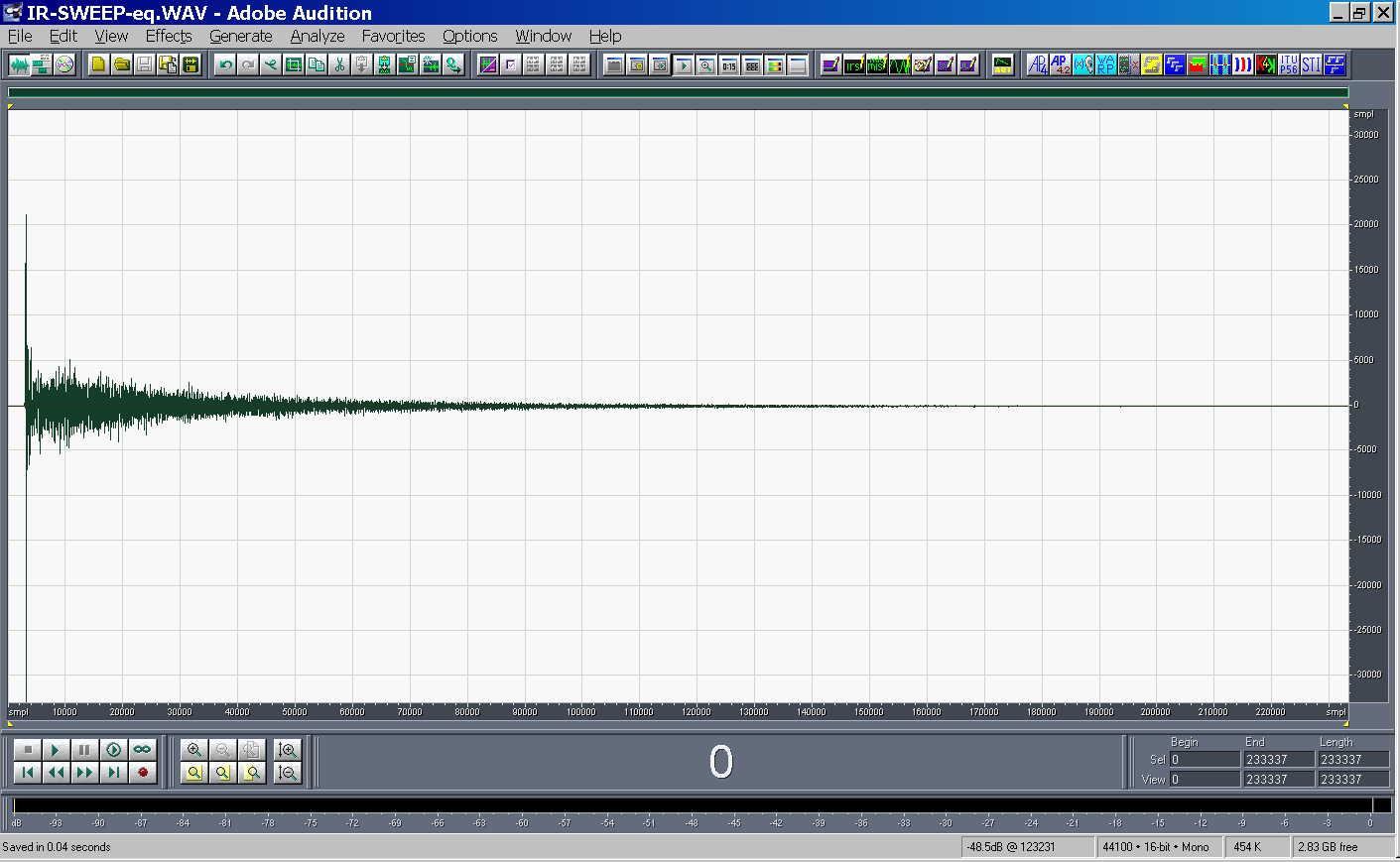
- The last impulse response is the linear one, the preceding are the
harmonics distortion products of various orders
|
|
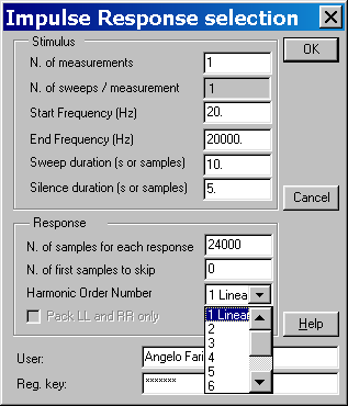
28
|
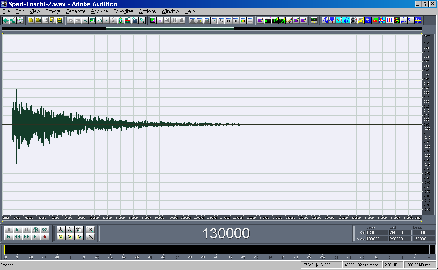
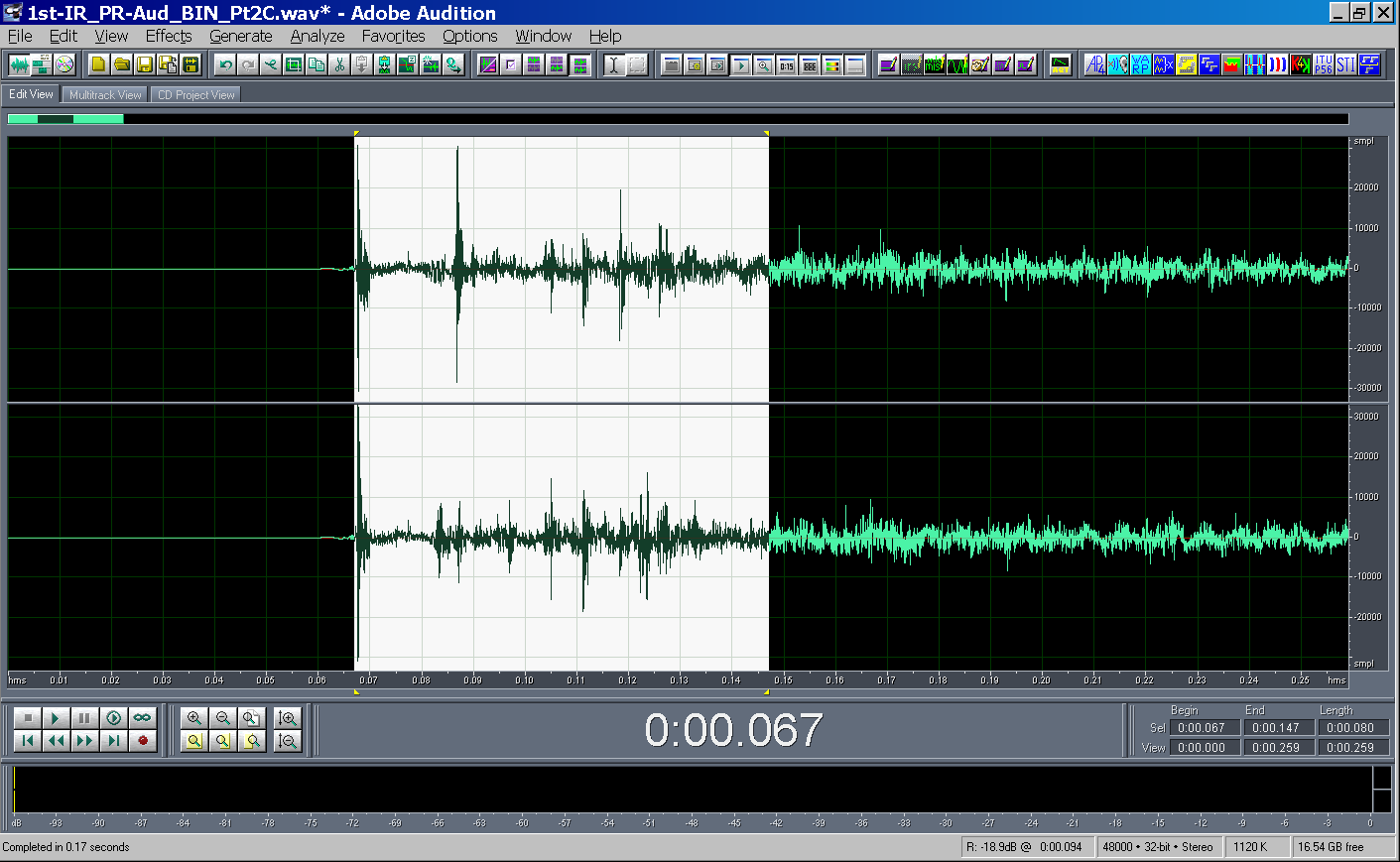
- After the sequence of impulse responses has been obtained, it is
possible to select and extract just one of them (the 1°-order - Linear
in this example):
|
|
29
|
|
|
30
|
|
|
31
|
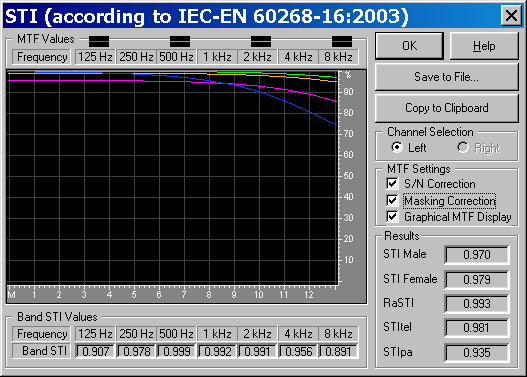
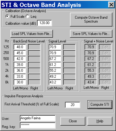
- A special plugin has been developed for the computation of STI according
to IEC-EN 60268-16:2003
|
|
32
|
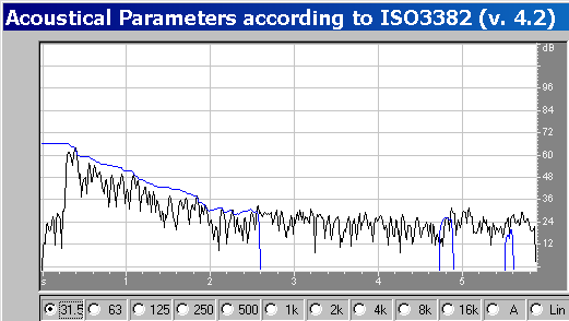
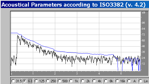
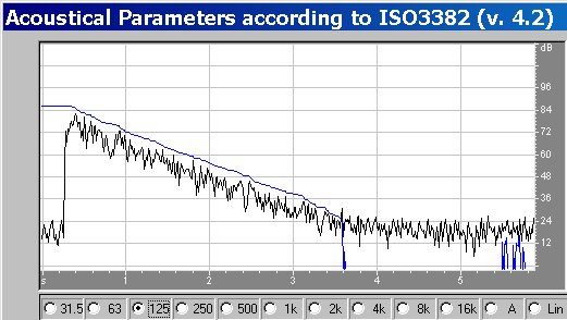
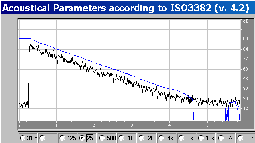
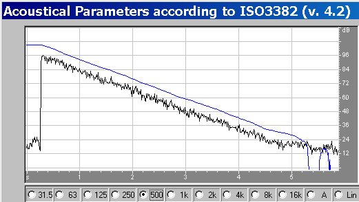
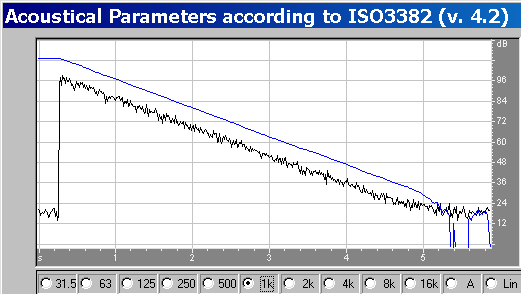
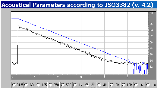
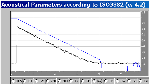
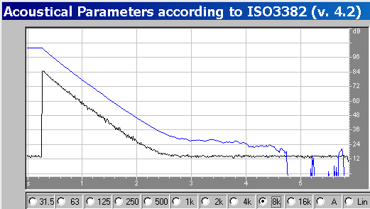
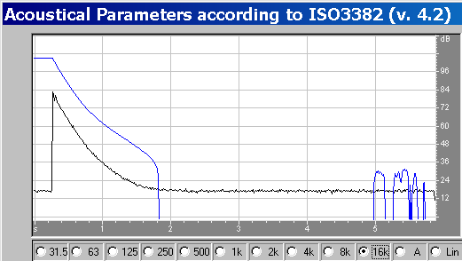
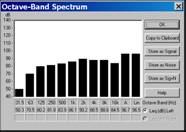
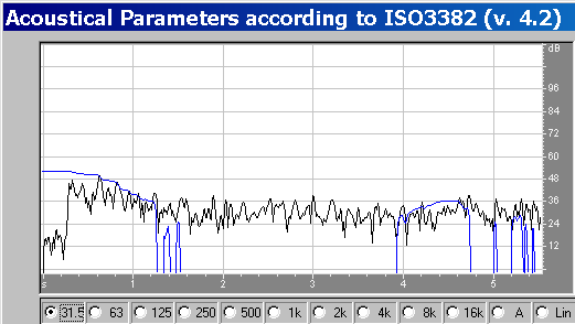
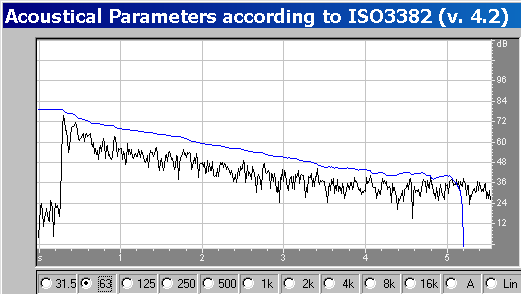
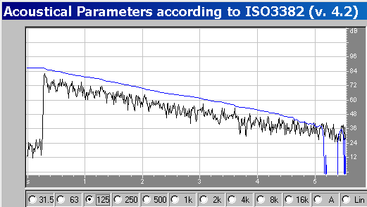
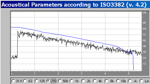
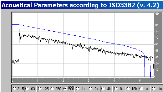
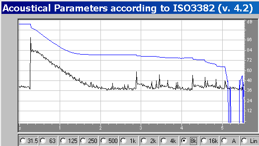
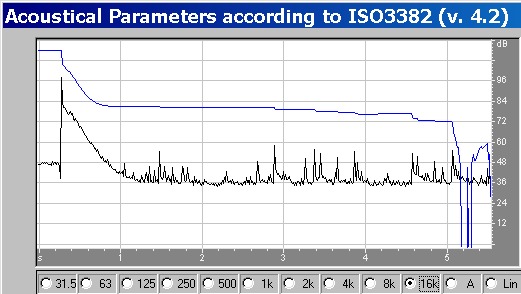
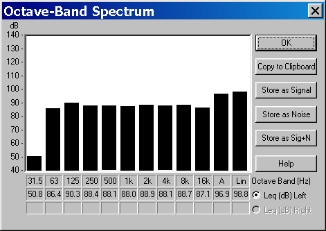
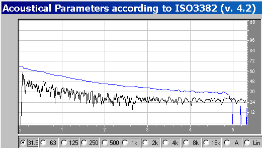
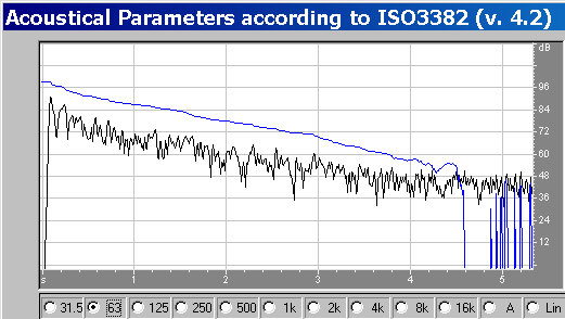
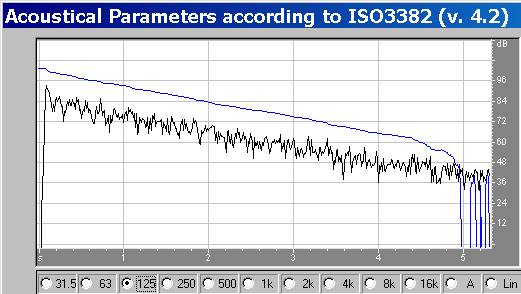
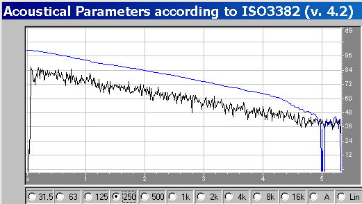
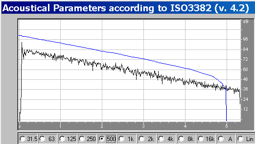
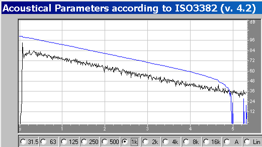
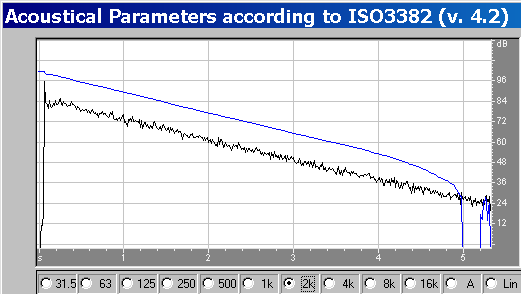
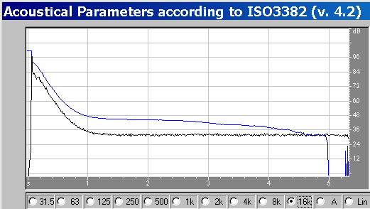
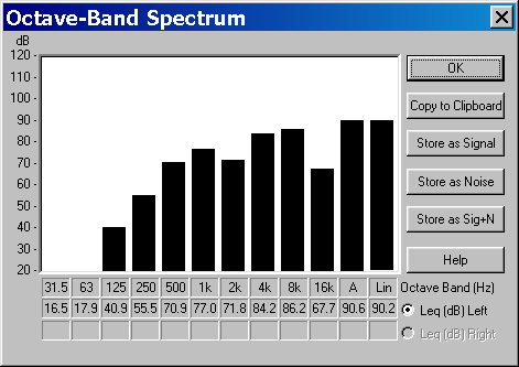
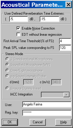
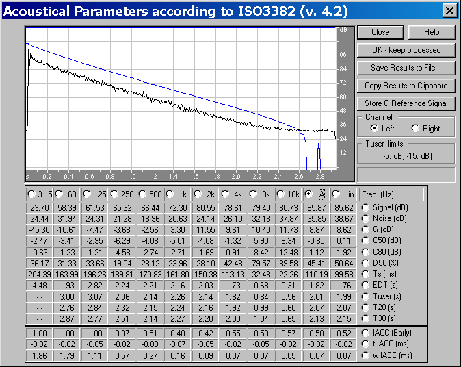
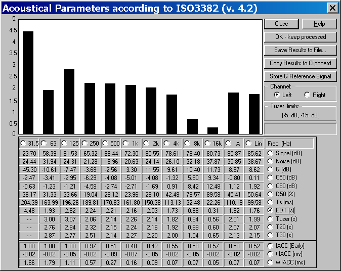
- A special plugin has been developed for performing analysis of
acoustical parameters according to ISO-3382
|
|
33
|
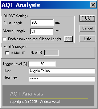
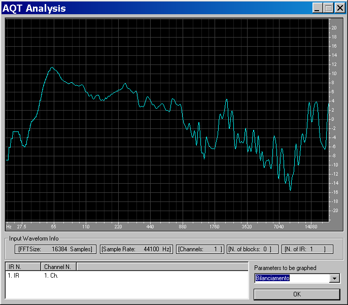
- The new module is still under development and will allow for very fast
computation of the AQT (Dynamic Frequency Response) curve from within
Adobe Audition
|
|
34
|
- The initial approach was to use directive microphones for gathering some
information about the spatial properties of the sound field “as
perceived by the listener”
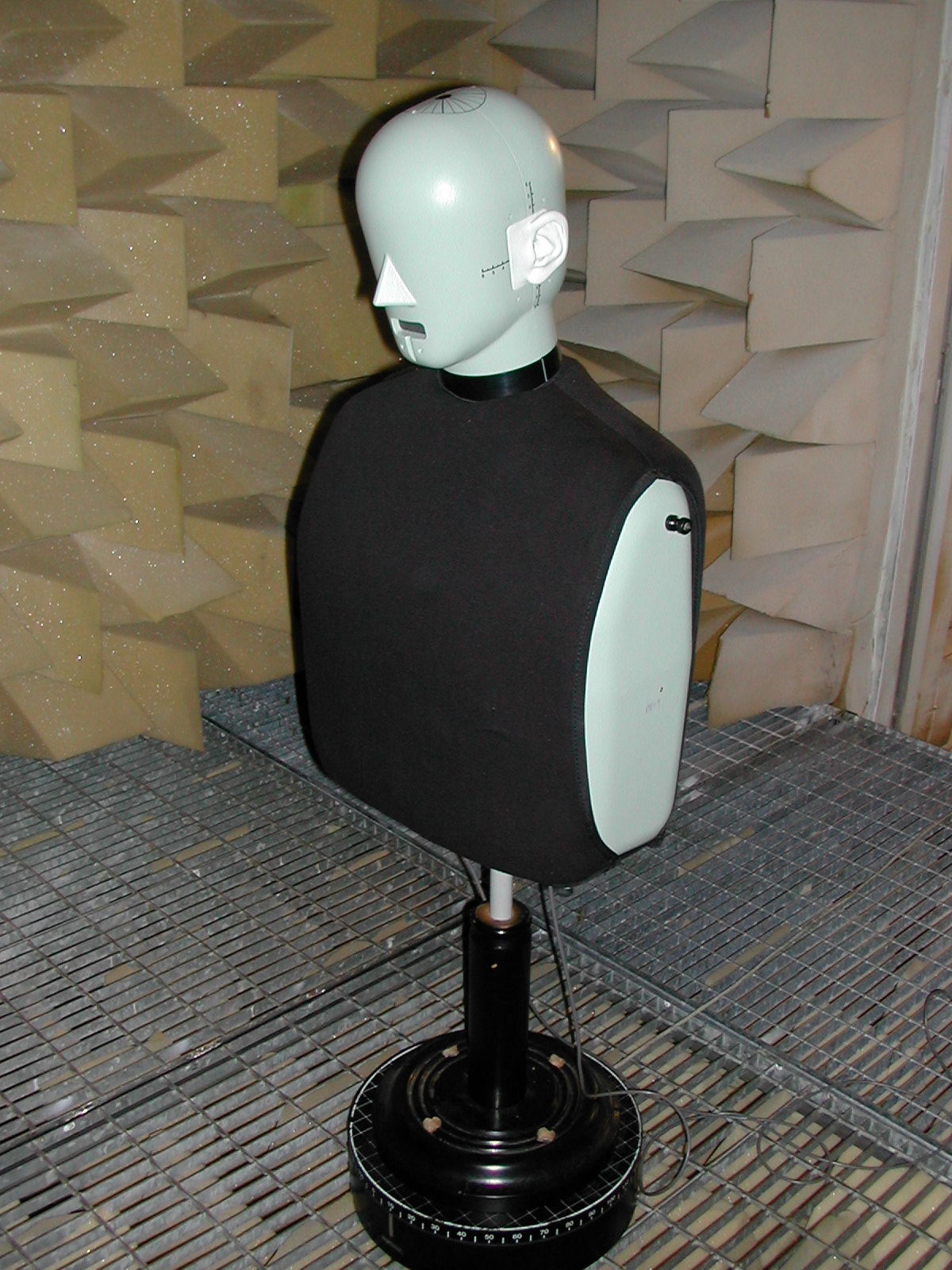
- Two apparently different approaches emerged: binaural dummy heads and
pressure-velocity microphones:
|
|
35
|
- It was attempted to “quantify” the “spatiality” of a room by means of
“objective” parameters, based on 2-channels impulse responses measured
with directive microphones
- The most famous “spatial” parameter is IACC (Inter Aural Cross
Correlation), based on binaural IR measurements
|
|
36
|
- Other “spatial” parameters are the Lateral Energy ratio LF
- This is defined from a 2-channels impulse response, the first channel is
a standard omni microphone, the second channel is a “figure-of-eight”
microphone:
|
|
37
|
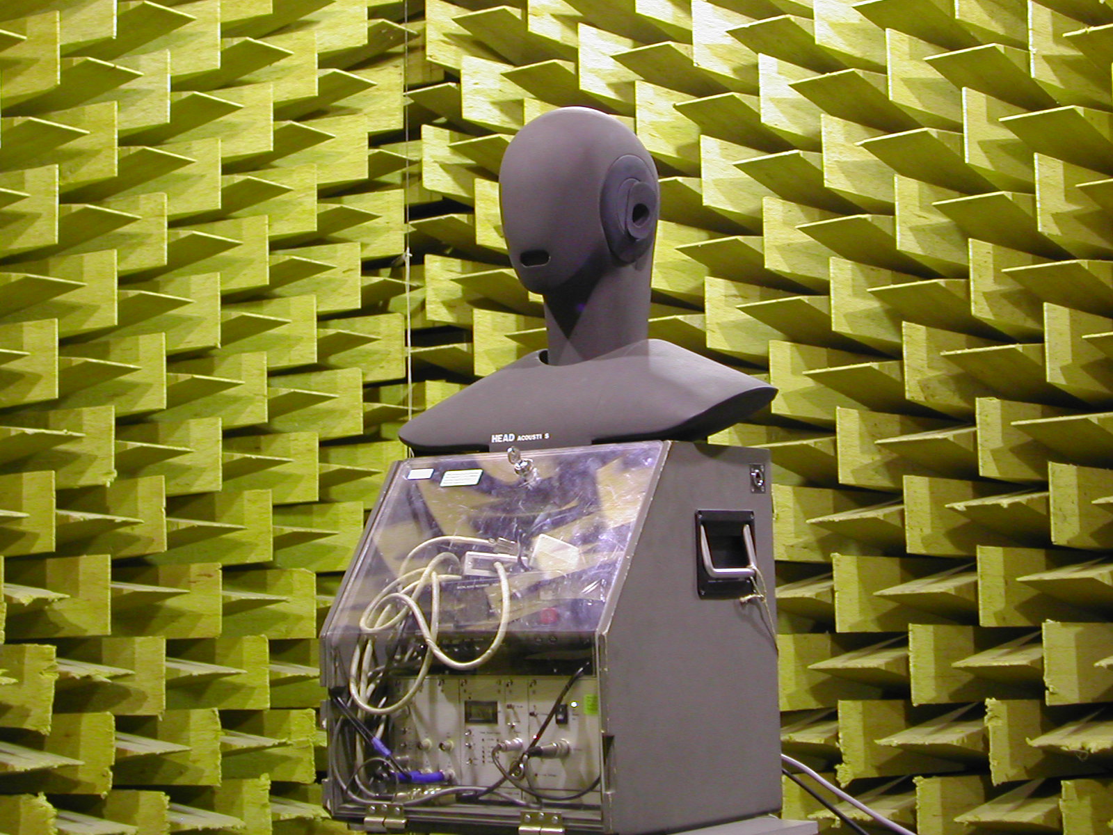
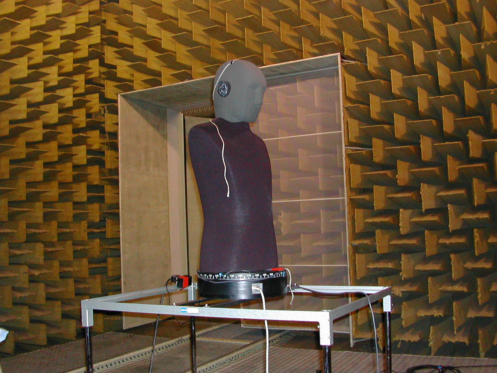
- Experiment performed in anechoic room - same loudspeaker, same source
and receiver positions, 5 binaural dummy heads
|
|
38
|
- Diffuse field - huge difference among the 4 dummy heads
|
|
39
|
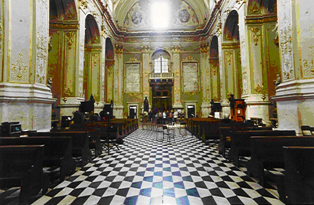
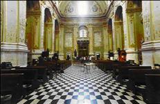
- Experiment performed in the Auditorium of Parma - same loudspeaker, same
source and receiver positions, 4 pressure-velocity microphones
|
|
40
|
- At 25 m distance, the scatter is really big
|
|
41
|
|
|
42
|
- The Soundfield microphone allows for simultaneous measurements of the
omnidirectional pressure and of the three cartesian components of
particle velocity (figure-of-8 patterns)
|
|
43
|
- The original idea of Michael Gerzon was finally put in practice in 2003,
thanks to the Israeli-based company WAVES
- More than 50 theatres all around the world were measured, capturing 3D
IRs (4-channels B-format with a Soundfield microphone)
- The measurments did also include binaural impulse responses, and a
circular-array of microphone positions
- More details on WWW.ACOUSTICS.NET
|
|
44
|
|
|
45
|
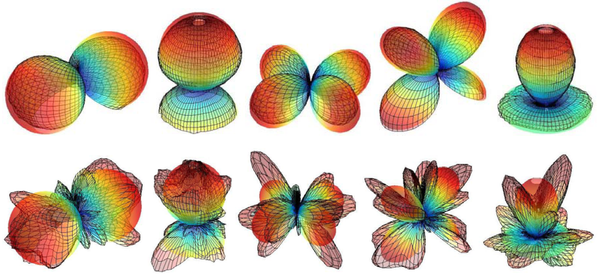
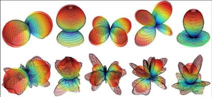
- Microphone arrays capable of synthesizing aribitrary directivity
patterns
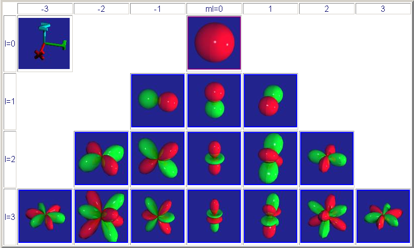
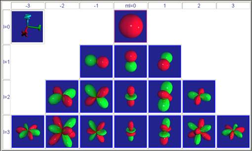
- Advanced spatial analysis of the sound field employing spherical
harmonics (Ambisonics - 1° order or higher)
- Loudspeaker arrays capable of synthesizing arbitrary directivity
patterns
- Generalized solution in which both the directivities of the source and
of the receiver are represented as a spherical harmonics expansion
|
|
46
|
|
|
47
|
- The answer is simple: analyze the spatial distribution of both source
and receiver by means of higher-order spherical harmonics expansion
- Spherical harmonics analysis is the equivalent, in space domain, of the
Fourier analysis in time domain
- As a complex time-domain waveform can be though as the sum of a number
of sinusoidal and cosinusoidal functions, so a complex spatial
distribution around a given notional point can be expressed as the sum
of a number of spherical harmonic functions
|
|
48
|
|
|
49
|
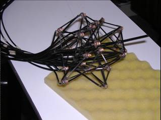
- Arnoud Laborie developed a 24-capsule compact microphone array - by
means of advanced digital filtering, spherical ahrmonic signals up to 3°
order are obtained (16 channels)
|
|
50
|
- Jerome Daniel and Sebastien Moreau built samples of 32-capsules
spherical arrays - these allow for extractions of microphone signals up
to 4° order (25 channels)
|
|
51
|
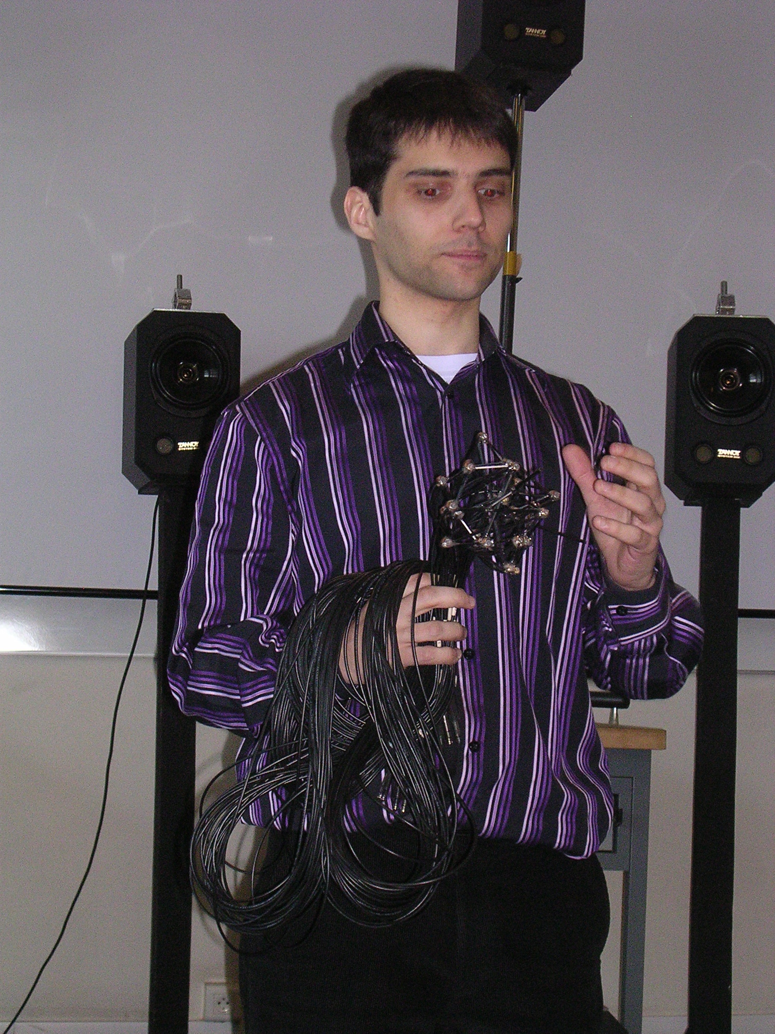
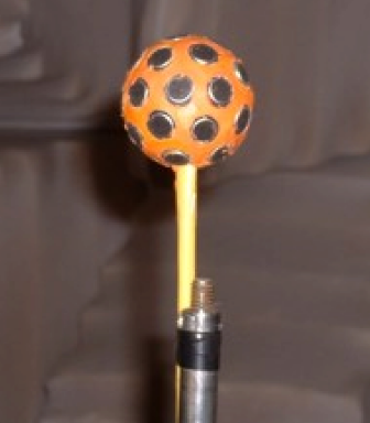
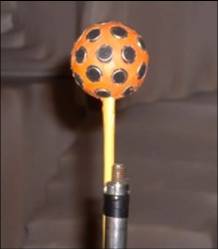
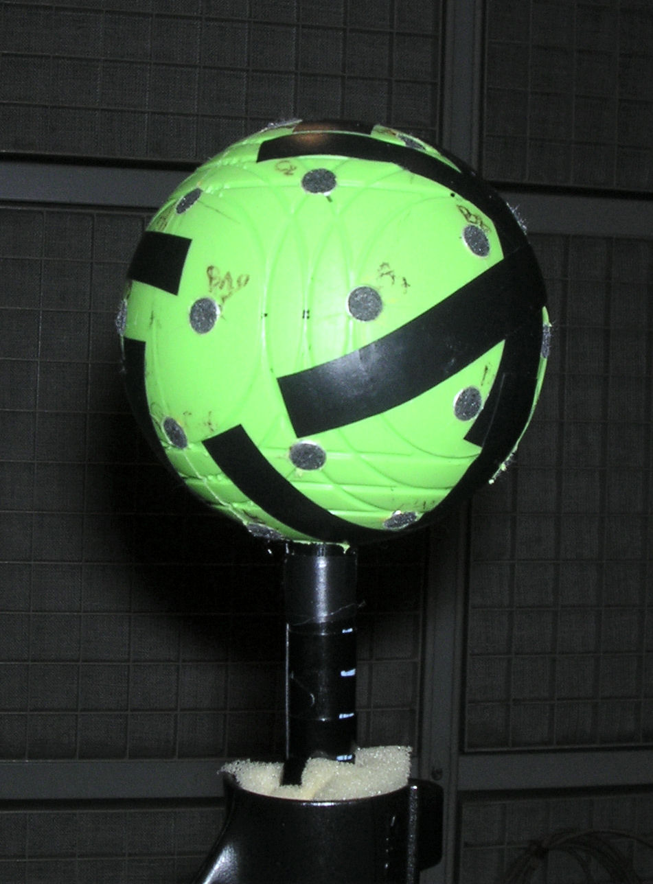
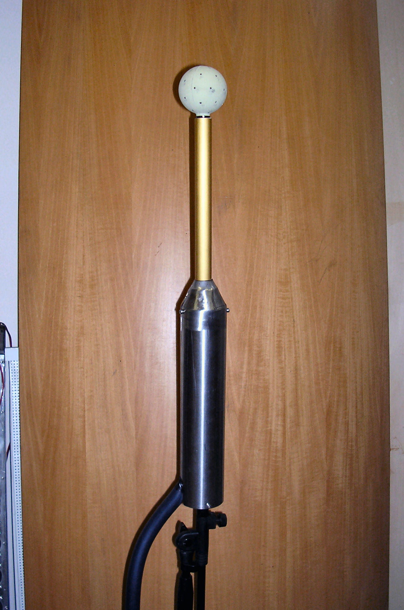
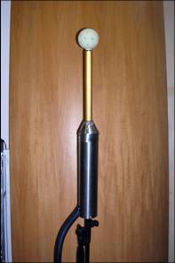
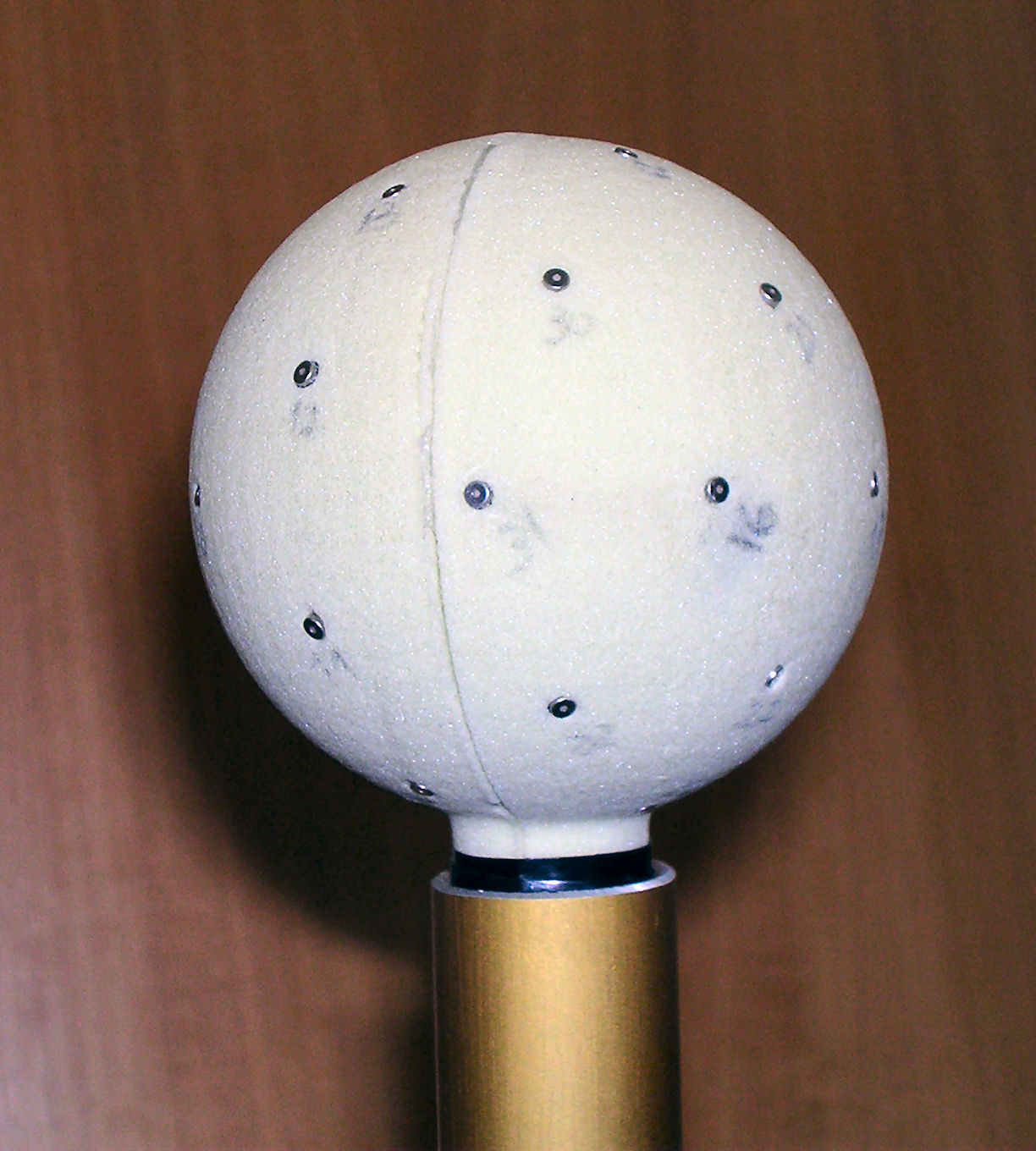
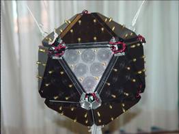
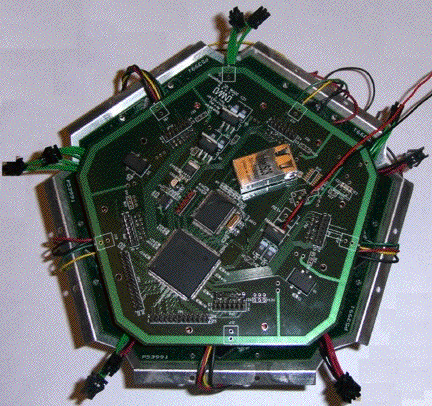
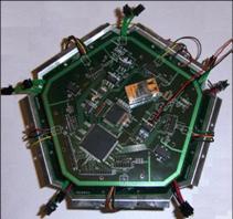
- Angelo Farina’s spherical mike (32 capsules)
|
|
52
|
- Chris Craig’s dual-sphere concentrical mike (64 capsules)
- And his 32-capsules cylindrical mike
|
|
53
|
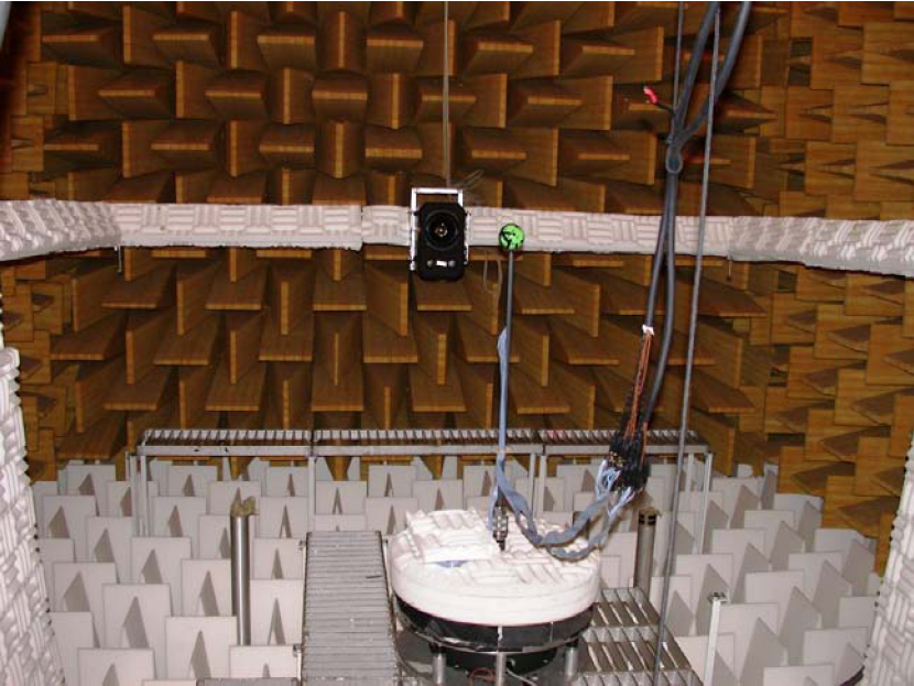
- Sebastien Moreau and Olivier Warusfel verified the directivity patterns
of their 4°-order microphone array in the anechoic room of IRCAM (Paris)
|
|
54
|
- Current 3D IR sampling is still based on the usage of an
“omnidirectional” source
- The knowledge of the 3D IR measured in this way provide no information
about the soundfield generated inside the room from a directive source
(i.e., a musical instrument, a singer, etc.)
- Dave Malham suggested to represent also the source directivity with a
set of spherical harmonics, called O-format - this is perfectly
reciprocal to the representation of the microphone directivity with the
B-format signals (Soundfield microphone).
- Consequently, a complete and reciprocal spatial transfer function can be
defined, employing a 4-channels O-format source and a 4-channels
B-format receiver:
|
|
55
|
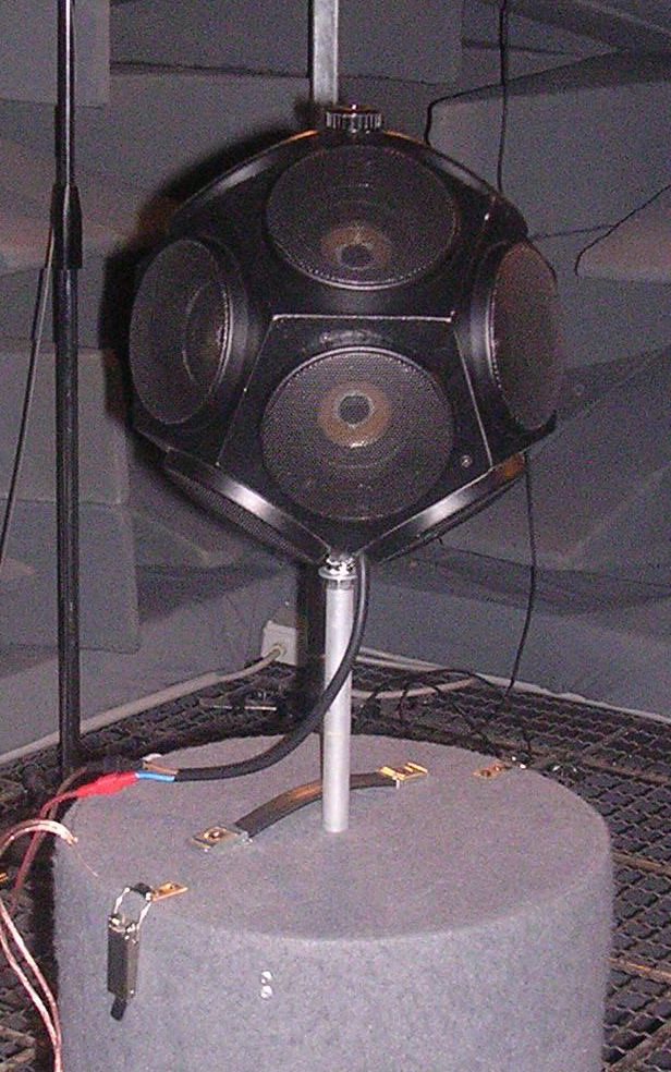
- LookLine D-300 dodechaedron
|
|
56
|
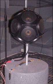
- LookLine D-200 dodechaedron
|
|
57
|
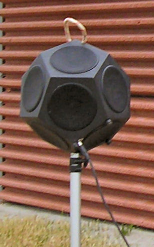
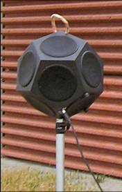
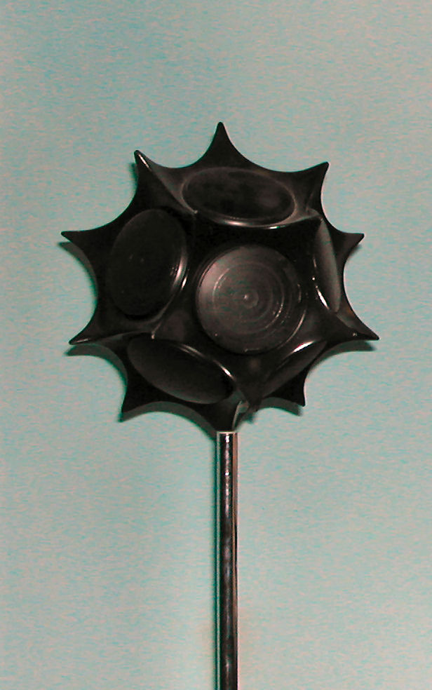
- Omnisonic 1000 dodechaedron
|
|
58
|
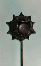
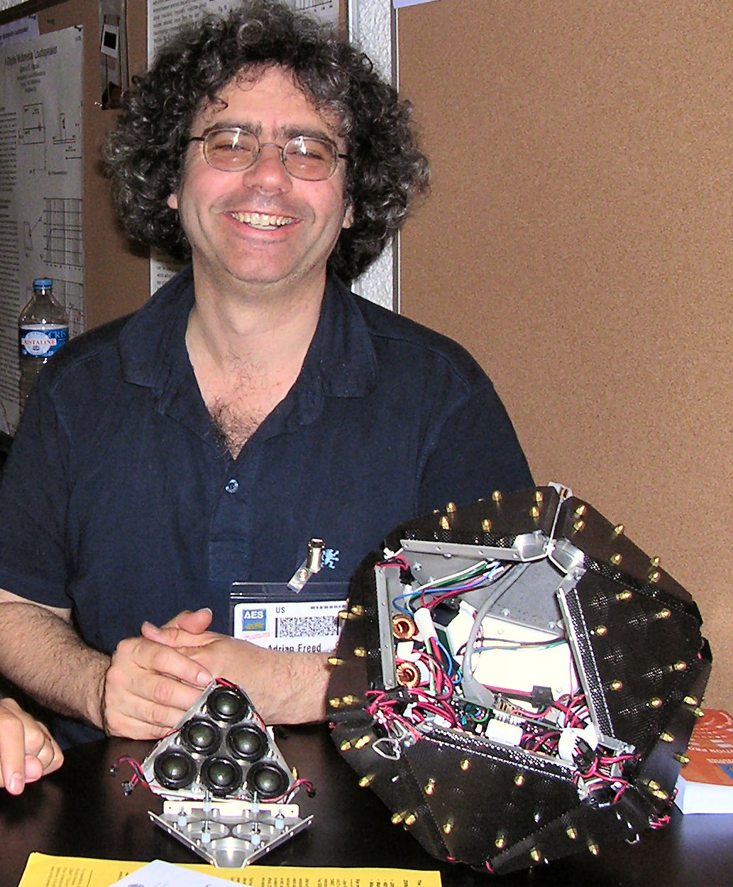
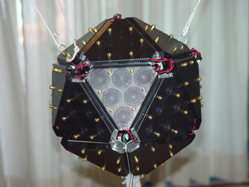
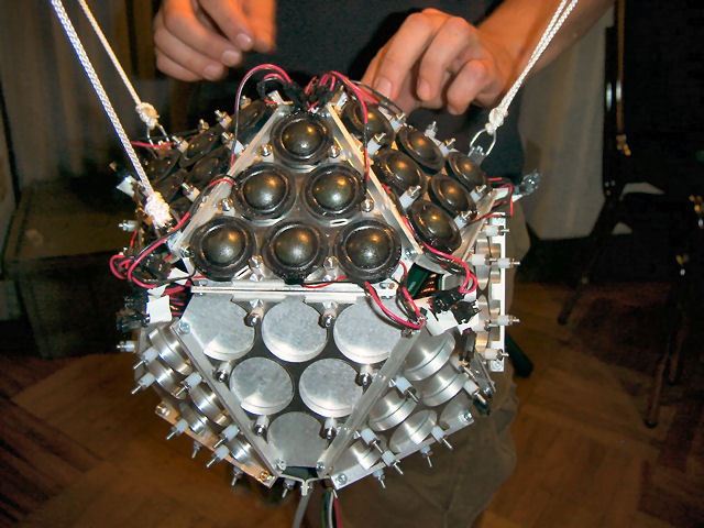
- Adrian Freed, Peter Kassakian, and David Wessel (CNMAT) developed a new
120-loudspeakers, digitally controlled sound source, capable of
synthesizing sound emission according to spherical harmonics patterns up
to 5° order.
|
|
59
|
- Class-D embedded amplifiers
|
|
60
|
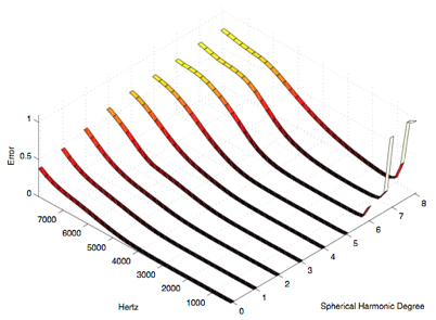
- The spatial reconstruction error of a 120-loudspeakers array is
frequency dependant, as shown here:
|
|
61
|
- Employing massive arrays of transducers, it will be feasible to sample
the acoustical temporal-spatial transfer function of a room
- Currently available hardware and software tools make this practical only
up to 4° order, which means 25 inputs and 25 outputs
- A complete measurement for a given source-receiver position pair takes
approximately 10 minutes (25 sine sweeps of 15s each are generated one
after the other, while all the microphone signals are sampled
simultaneously)
- However, it has been seen that real-world sources can be already
approximated quite well with 2°-order functions, and even the human HRTF
directivites are reasonally approximated with 3°-order functions.
|
|
62
|
|
|
63
|
|
|
64
|
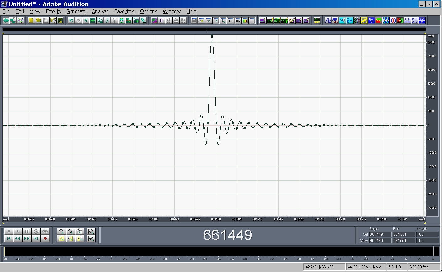
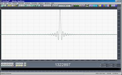
- Pre-ringing at high frequency due to improper fade-out
|
|
65
|
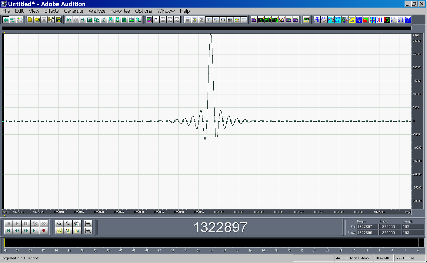
- Perfect Dirac’s delta after removing the fade-out
|
|
66
|
- Pre-ringing at low frequency due to a bad sound card featuring
frequency-dependent latency
|
|
67
|
- The Kirkeby inverse filter is computed inverting the measured IR
|
|
68
|
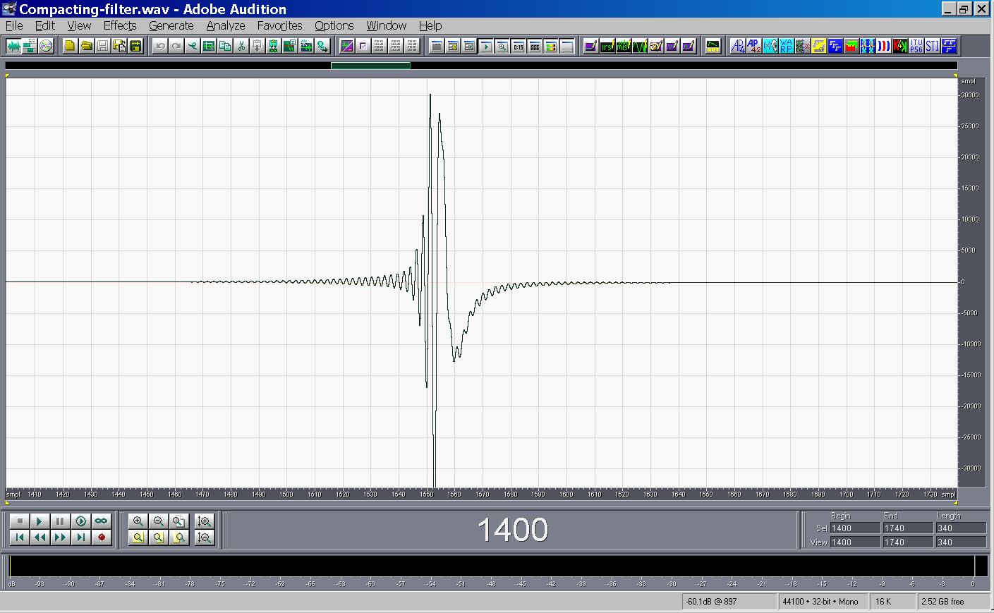
- Convolving the time-smeared IR with the Kirkeby compacting filter, a
very sharp IR is obtained
|
|
69
|
|
|
70
|
- An anechoic measurement is first performed
|
|
71
|
- A suitable inverse filter is generated with the Kirkeby method by
inverting the anechoic measurement
|
|
72
|
- The inverse filter can be either pre-convolved with the test signal or
post-convolved with the result of the measurement
- Pre-convolution usually reduces the SPL being generated by the
loudspeaker, resulting in worst S/N ratio
- On the other hand, post-convolution can make the background noise to
become “coloured”, and hence more perciptible
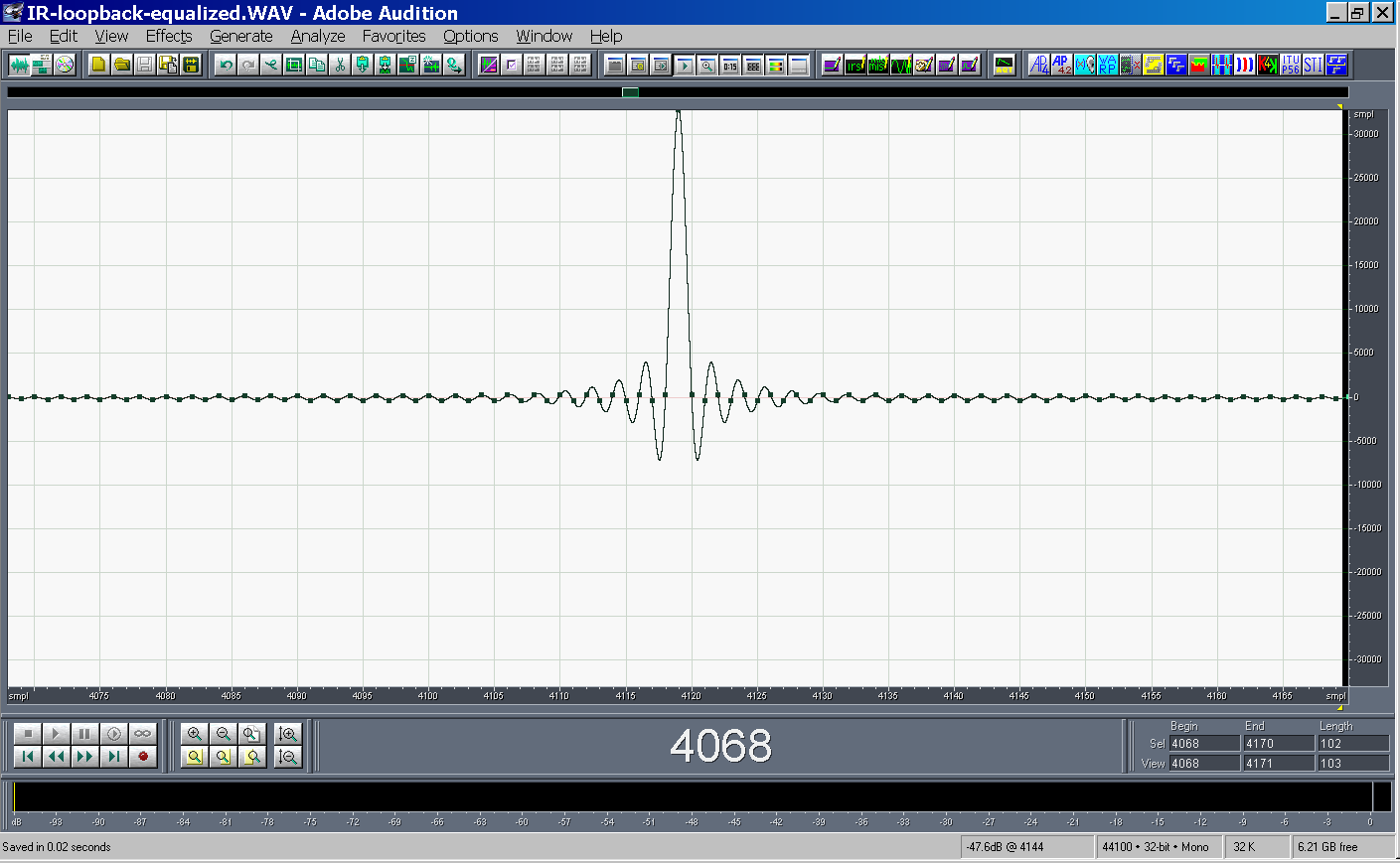
- The resulting anechoic IR becomes almost perfectly a Dirac’s Delta
function:
|
|
73
|
|
|
74
|
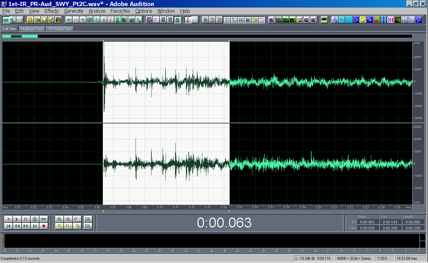
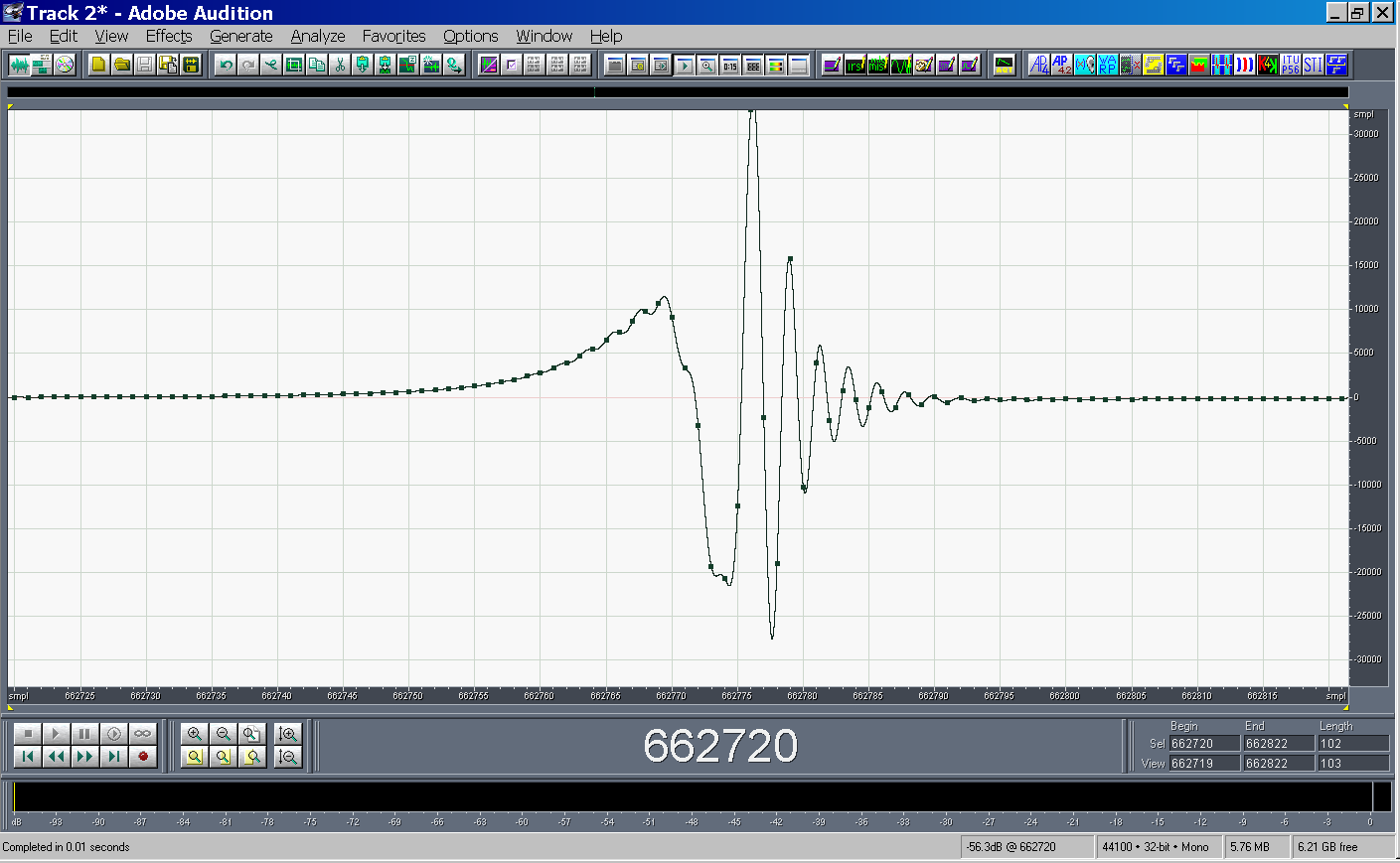
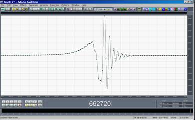
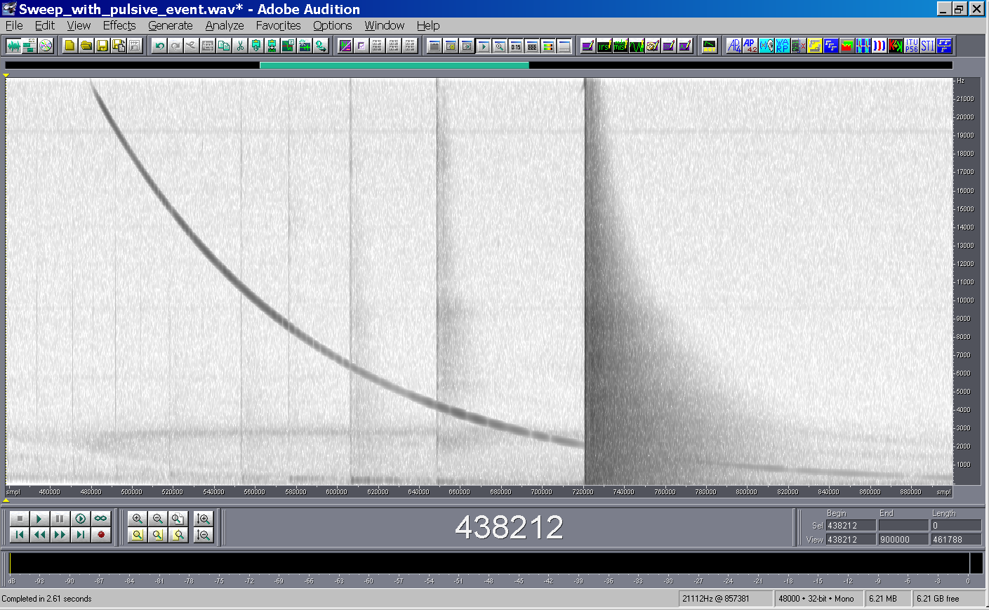
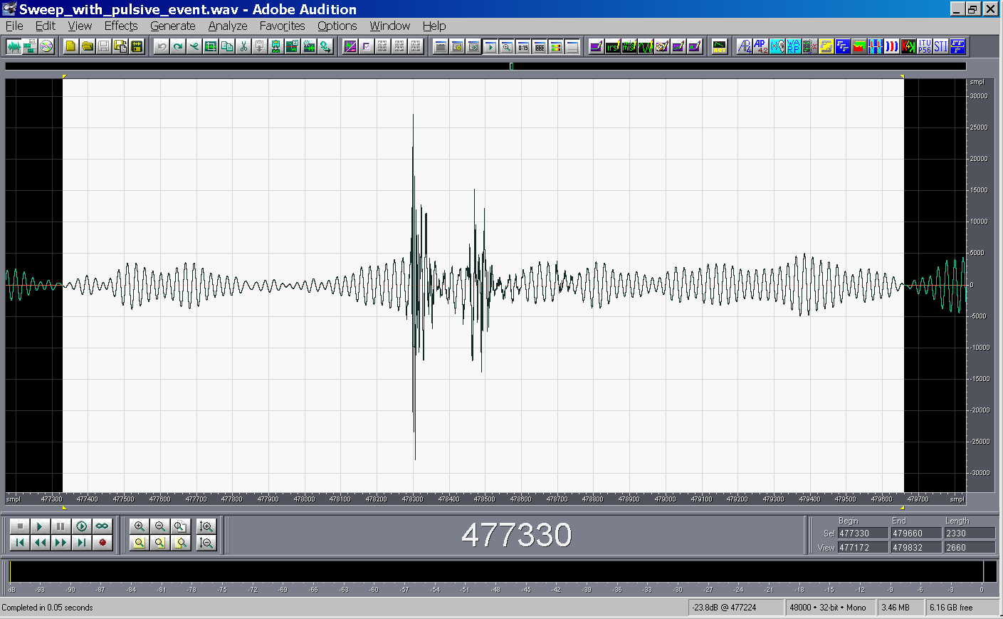
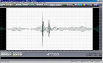
- Often a pulsive noise occurs during a sine sweep measurement
|
|
75
|
- After deconvolution, the pulsive sound causes untolerable artifacts in
the impulse response
|
|
76
|
- Several denoising techniques can be employed:
- Brutely silencing the transient noise
- Employing the specific “click-pop eliminator” plugin of Adobe Audition
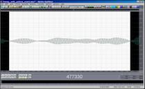
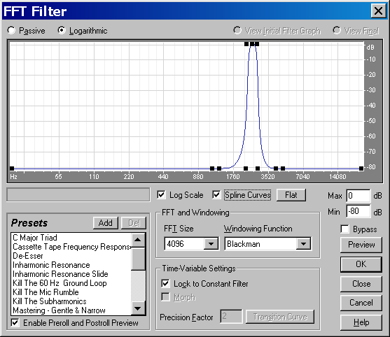
- Applying a narrow-passband filter around the frequency which was being
generated in the moment in which the pulsive noise occurred
- The third approach provides the better results:
|
|
77
|
|
|
78
|
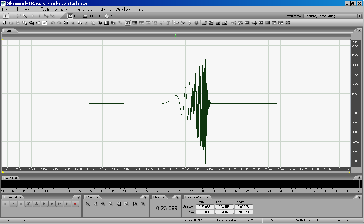
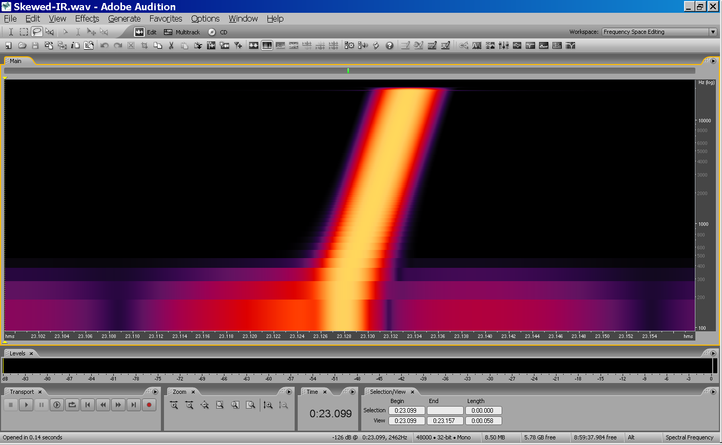
- When the measurement is performed employing devices which exhibit
signifcant clock mismatch between playback and recording, the resulting
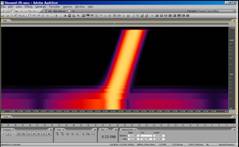
impulse response is “skewed” (stretched in time):
|
|
79
|
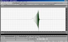
- It is possible to re-pack the impulse response employing the
already-described approach based on the usage of a Kirkeby inverse
filter:
|
|
80
|
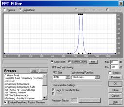
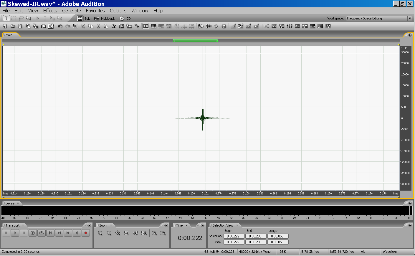
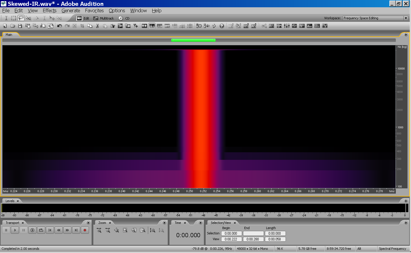
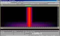
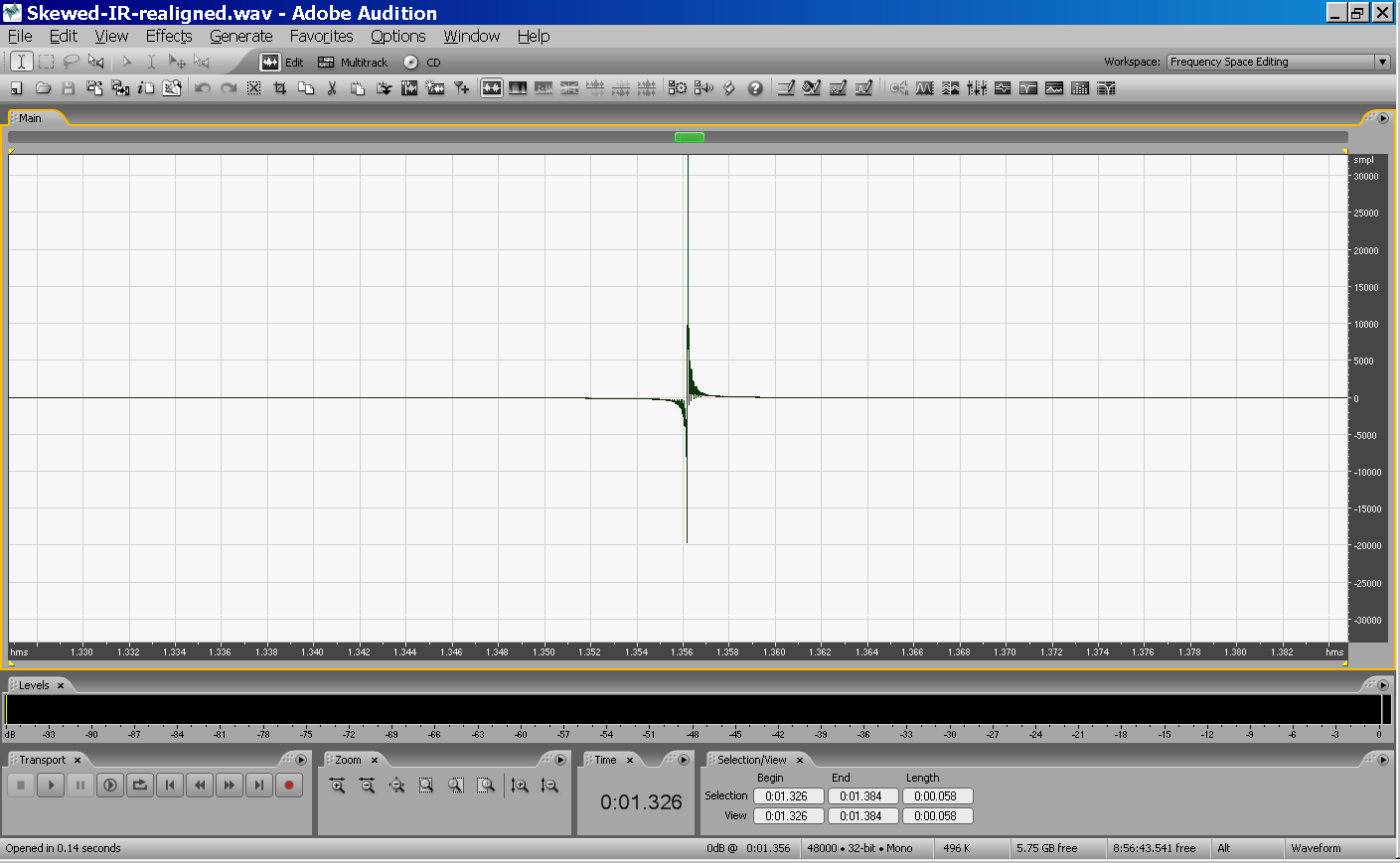
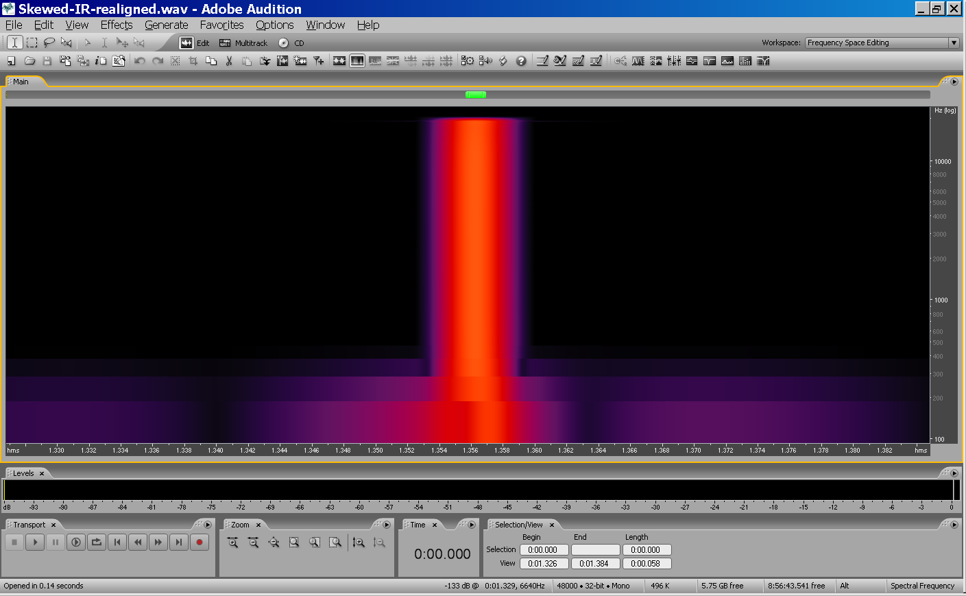
- However, it is always possible to generate a pre-stretched inverse
filter, which is longer or shorter than the “theoretical” one - by
proper selection of the lenght of the inverse filter, it is possible to
deconvolve impulse responses which are almost perfectly “unskewed”:
|
|
81
|
|
|
82
|
- When several impulse response measurements are synchronously-averaged
for improving the S/N ratio, the late part of the tail cancels out,
particularly at high frequency, due to slight time variance of the
system
|
|
83
|
- However, if averagaing is performed properly in spectral domain, and a
single conversion to time domain is performed after averaging, this
artifact is significantly reduced
- The new “cross Functions” plugin can be used for computing H1:
|
|
84
|
- The ESS method revealed to be systematically superior to the MLS method
for measuring electroacoustical impulse responses
- Traditional methods for measuring “spatial parameters” (IACC, LF) proved
to be unreliable and do not provide complete information
- The 1°-order Ambisonics method can be used for generating and recording
sound with a limited amount of spatial information
- For obtaining better spatial resolution, High-Order Ambisonics can be
used, limiting the spherical-harmonics expansion to a reasonable order
(2°, 3° or 4°).
- Experimental hardware and software tools have been developed (mainly in
France, but also in USA), allowing to build an inexpensive complete
measurement system
|
|
85
|
- ESS is now employed in top-grade measurement systems:
Audio Precision (TM), Rhode-Schwartz and B&K / DIRAC
- However, these completely-packaged measurement systems often do not
allow to play “tricks” and to adjust the signals for solving problems,
which have been shown here
- Workarounds have been found for the problems occurring when performing
ESS measurements
- These workarounds are easily applied by working with a general purpose
sound editor (Adobe Audition)
- A number of additional plugins have been developed, making easy to
generate the test signal, to deconvolve and process impulse responses,
to compute inverse filters and to perform advanced processing (STI, AQT,
etc.)
- These plugins are freely downlodable at the AURORA web site:
- www.aurora-plugins.com
|

 Notes
Notes