|
1
|
- Angelo Farina, Enrico Armelloni
- Industrial Engineering Dept., University of Parma, Via delle Scienze
181/A
- Parma, 43100 ITALY – HTTP://pcfarina.eng.unipr.it
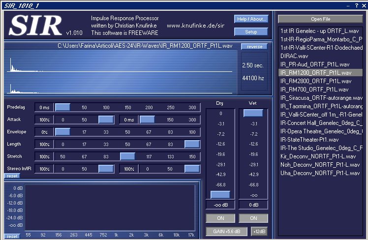
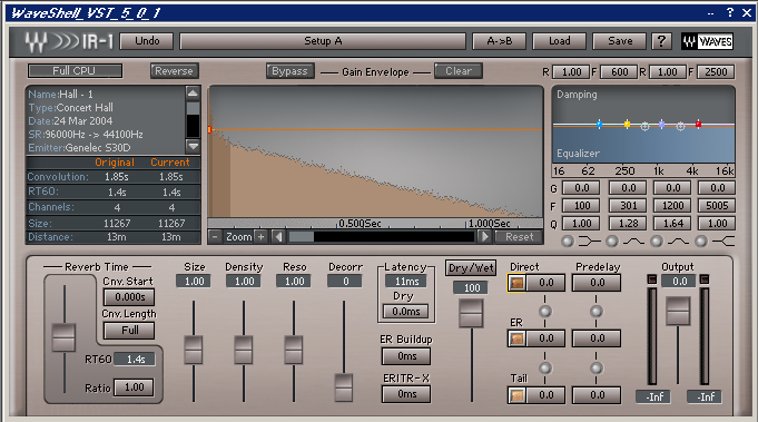
|
|
2
|
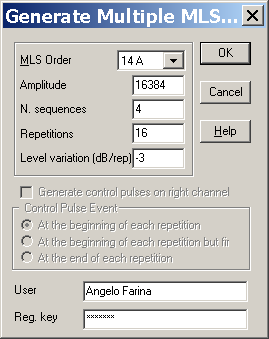
- Transform the results of objective electroacoustics measurements to
audible sound samples suitable for listening tests
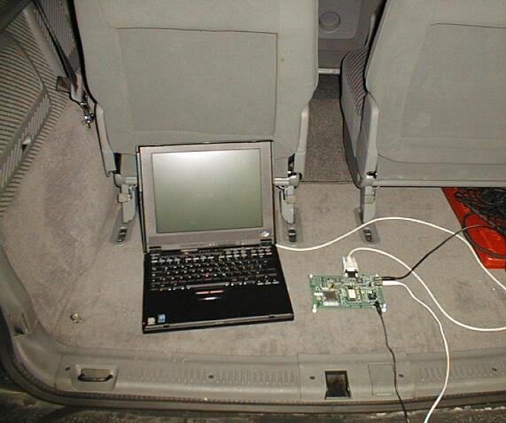
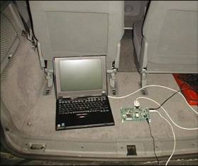
|
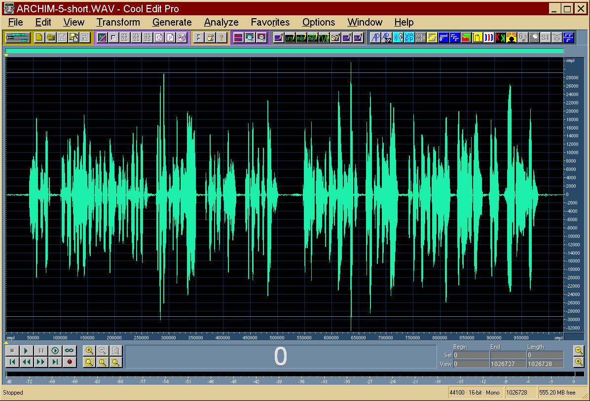
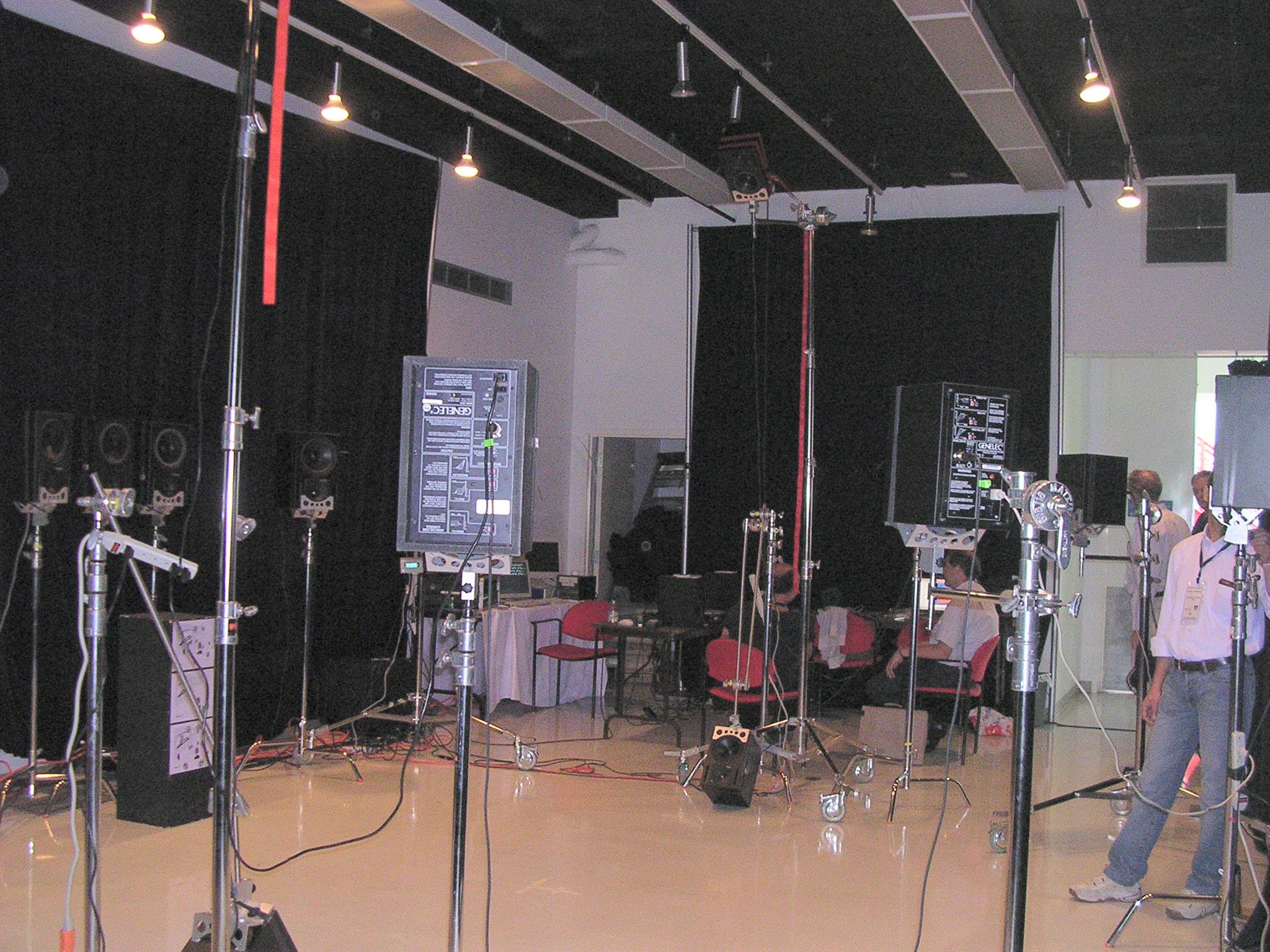
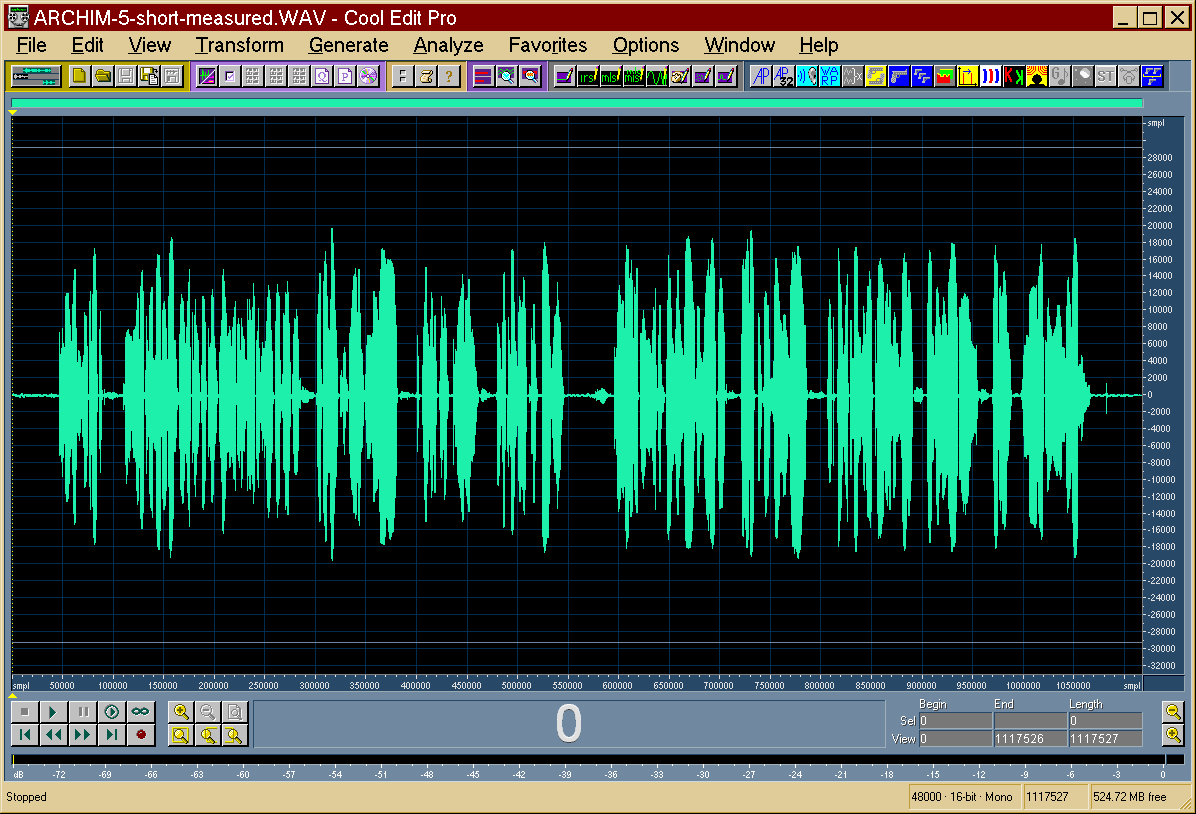
|
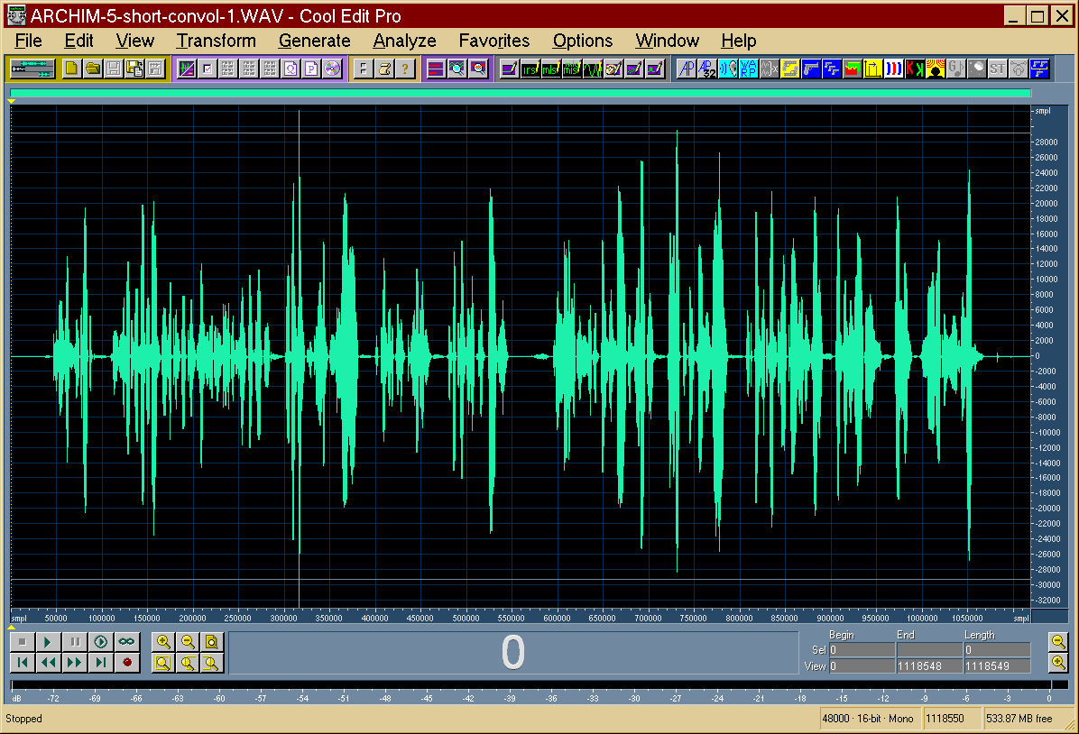
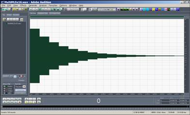
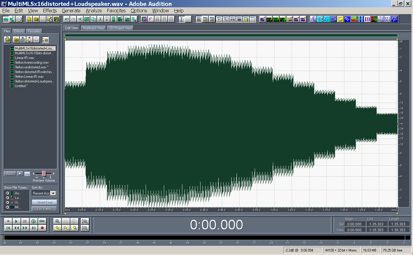
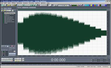
3
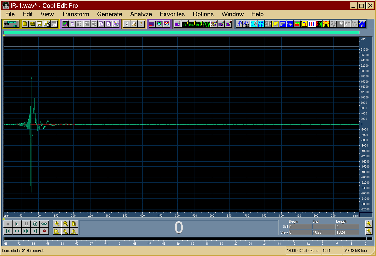
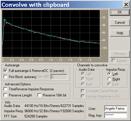
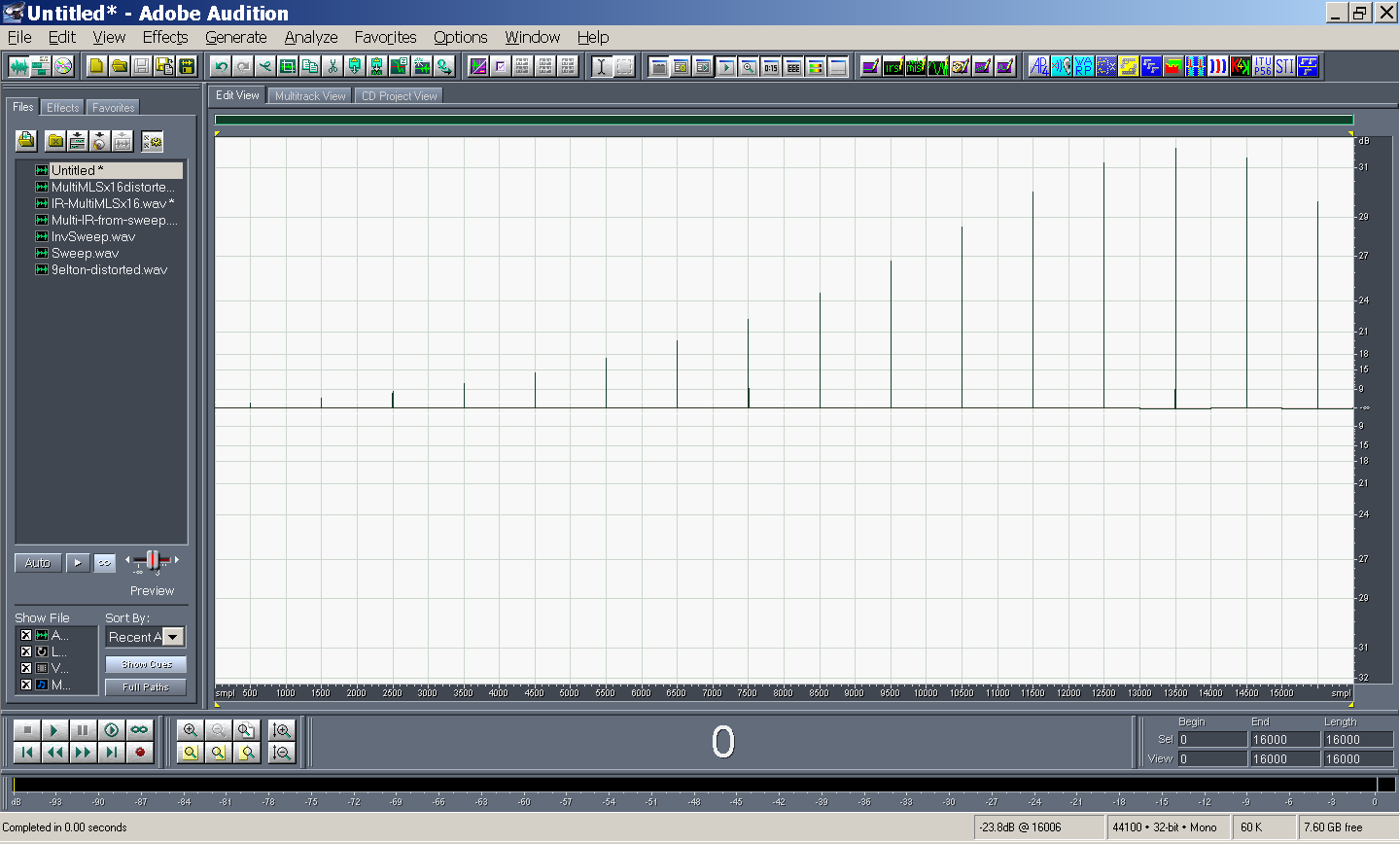
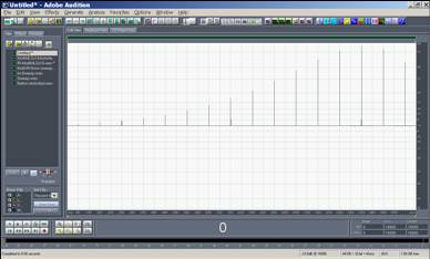
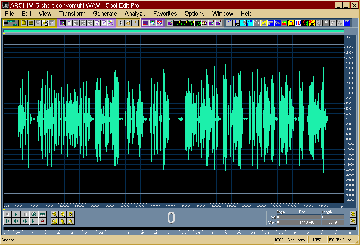
|
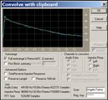
- Convolving a suitable sound sample with the linear IR, the frequency
response and temporal transient effects of the system can be simulated
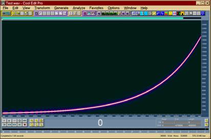
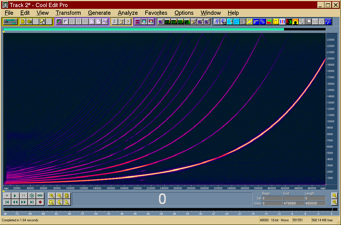
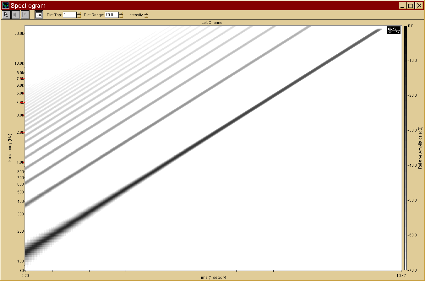
properly
|
|
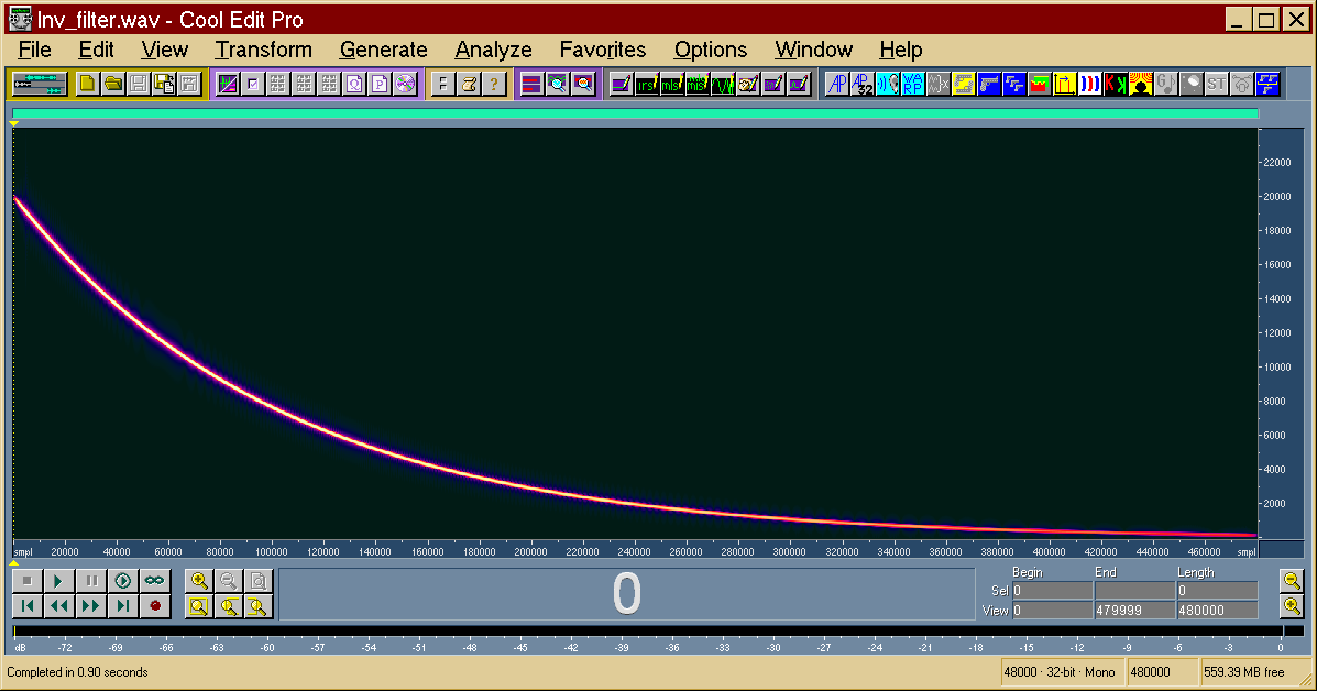
4
|
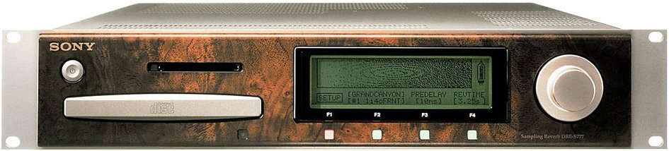
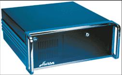
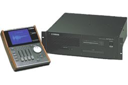
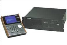
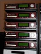
- The beginnings: hardware DSP-based convolution units
|
|
5
|
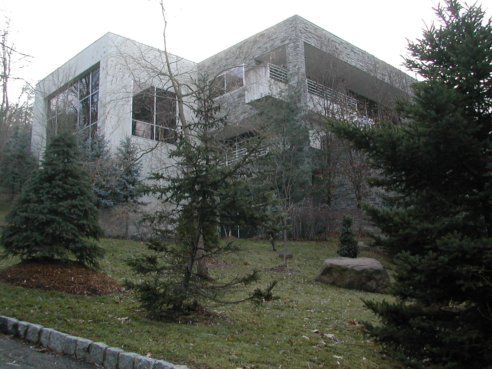
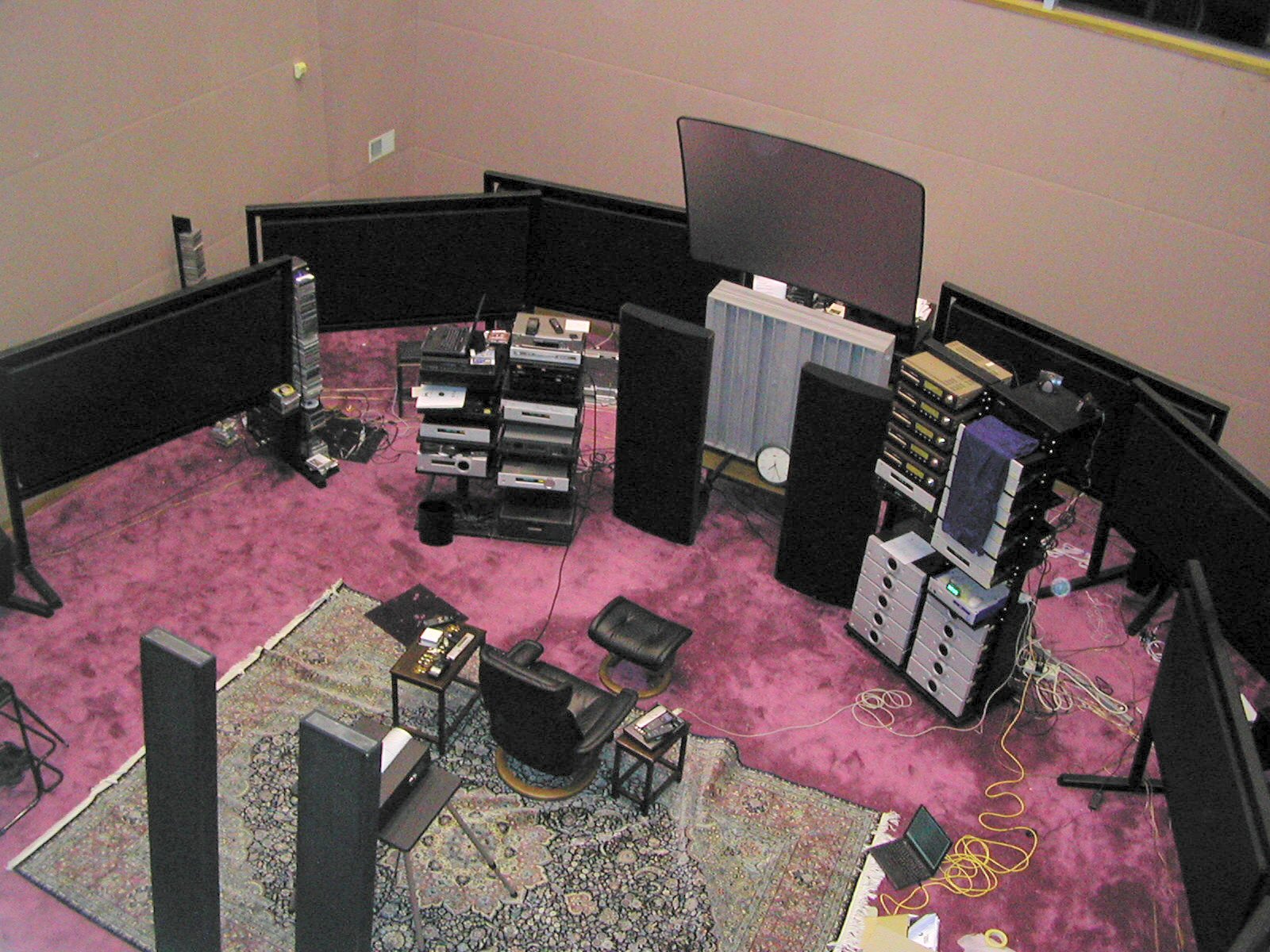
- The AMBIOPHONICS Institute: the home of convolution
|
|
6
|
- Open-source software for Linux by Anders Torger – AES 24° Conference
|
|
7
|
- Nowadays many sytems or software plugins can perform satisfactorily the
Linear Convolution operation, and are widely employed for audio
processing
|
|
8
|
- No harmonic distortion, nor other nonlinear effects are being reproduced.
- From a perceptual point of view,
the sound is judged “cold” and “innatural”
- A comparative test between a strongly nonlinear device and an almost
linear one does not reveal any audible difference, because the nonlinear
behavior is removed for both
|
|
9
|
- A very simple idea: a different IR is employed depending on the
amplitude of each sample of the signal to be filtered
- The method is quite old: the first published papers are thoss of Bellini
and Farina (1988) and Michael Kemp (1999)
- Several impulse responses are measured, employing test signals of
different amplitudes, and stored for later usage.
- It is mandatory to implement the convolution as direct form in time
domain, as each sample has to be processed with a different IR.
|
|
10
|
- Michael Kemp employed a step function, with several steps of decreasing
amplitude
|
|
11
|
- Farina e Bellini did employ a sequence of MLS repetitions, each with
decreasing amplitude
|
|
12
|
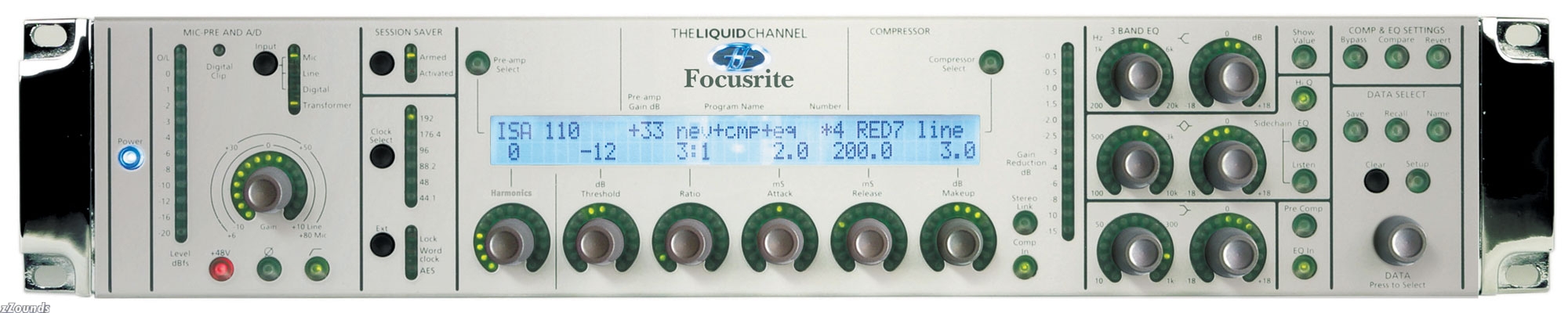
- Focusrite did release recently Liquid Channel, the first “dynamic
convolver” implementing the IR-switching technique
|
|
13
|
- A FIR filtering algorithm, with the set of coefficients chosen depending
on the sample amplitude, was implemented on a Sharc EZ-KIT 20161 board,
and employed for car-audio applications
|
|
14
|
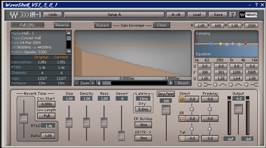
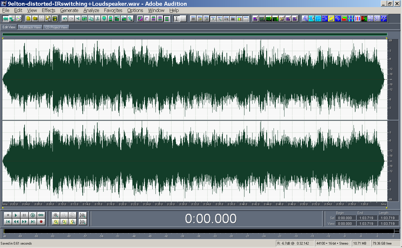
- The “not linear device” is emulated by the DISTORTION plugin of Adobe Audition,
followed by sound playback and simultaneous recording over the
loudspeaker and microphone of a laptop PC
|
|
15
|
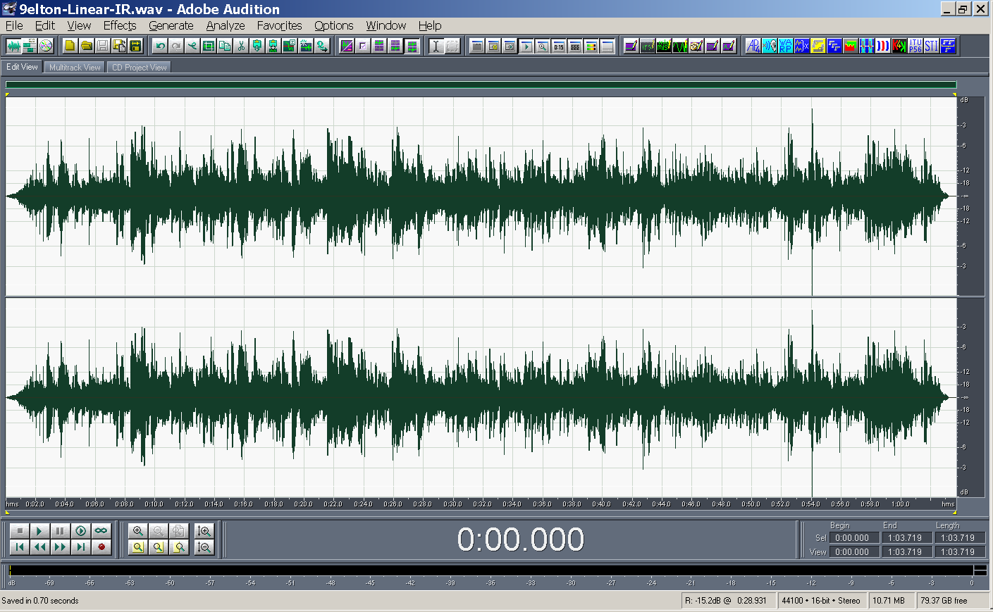
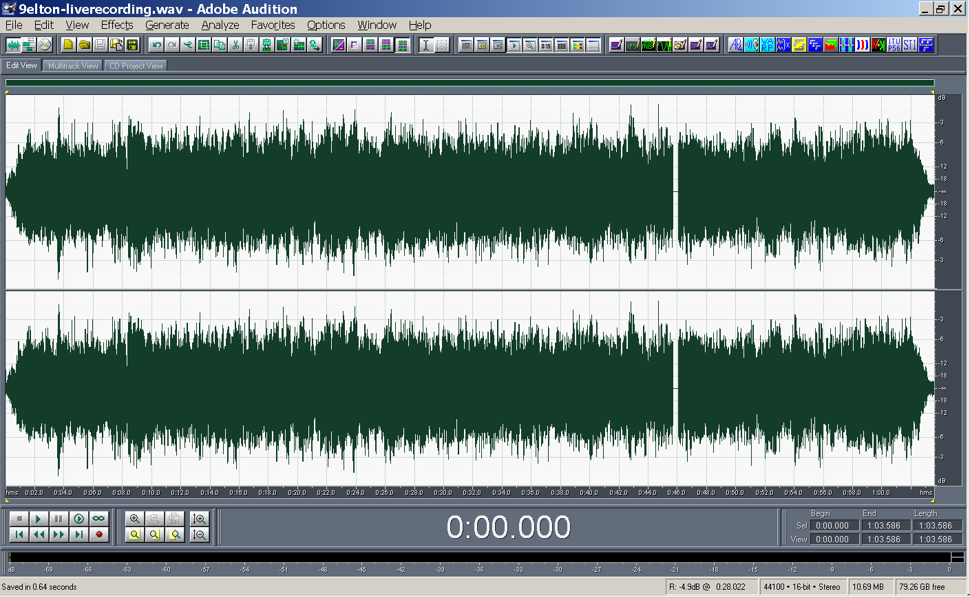
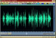
- This is the multiple MLS signals after being processed through the
not-linear device
|
|
16
|
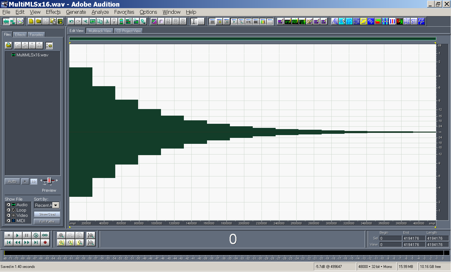
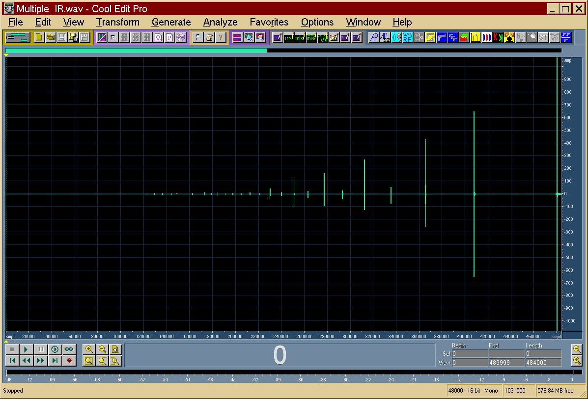
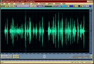
- Here the 16 impulse responses measured with MLS of different amplitude
(decreasing 3dB each from left to right) are shown
|
|
17
|
|
|
18
|
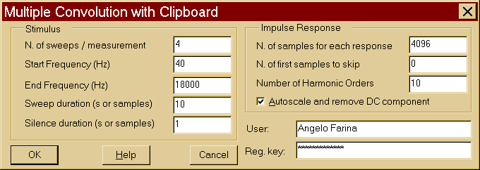
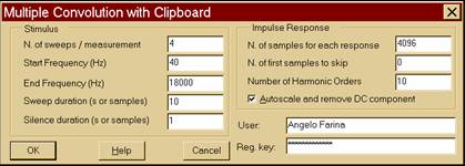
- We start from a measurement of the system based on exponential sine
sweep (Farina, 108th AES, Paris 2000)
- Diagonal Volterra kernels are obtained by post-processing the
measurement results
- These kernels are employed as FIR filters in a multiple-order
convolution process (original signal, its square, its cube, and so on
are convolved separately and the result is summed)
|
|
19
|
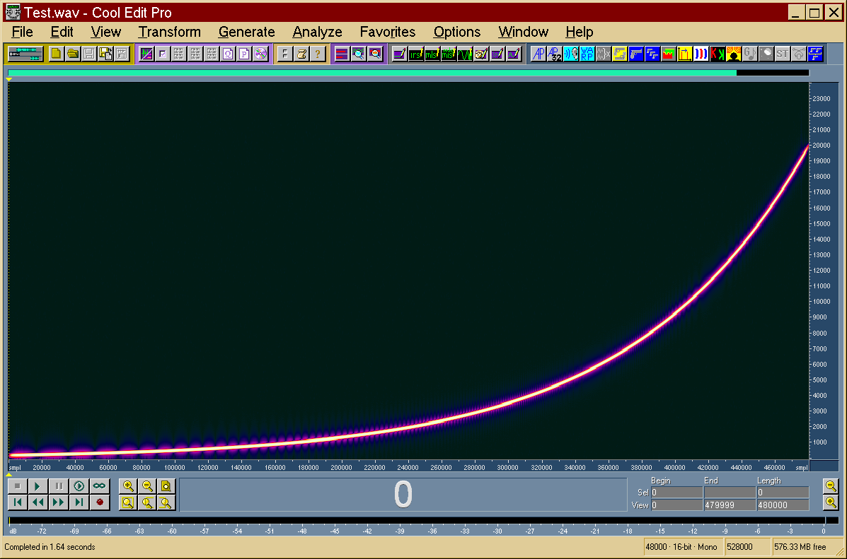
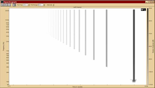
- The test signal is a sine sweep with constant amplitude and
exponentially-increasing frequency
|
|
20
|
- Many harmonic orders do appear as colour stripes
|
|
21
|
- Many harmonic orders do appear as colour stripes
|
|
22
|
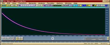
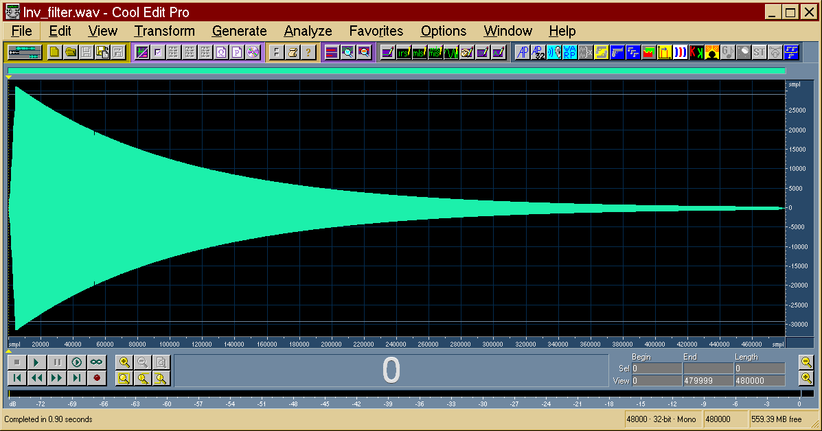
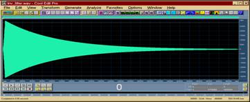
- The deconvolution is obtained by convolving the raw response with a
suitable inverse filter
|
|
23
|
- The last peak is the linear impulse response, the preceding ones are the
harmonic distortion orders
|
|
24
|
- The last peak is the linear impulse response, the preceding ones are the
harmonic distortion orders
|
|
25
|
- The basic approach is to convolve separately, and then add the result,
the linear IR, the second order IR, the third order IR, and so on.
- Each order IR is convolved with the input signal raised at the
corresponding power:
|
|
26
|
- The general Volterra series expansion is defined as:
|
|
27
|
- The first nonlinear system is assumed to be memory-less, so only the
diagonal terms of the Volterra kernels need to be taken into account.
|
|
28
|
- The measured multiple IRs h’ can be defined as:
|
|
29
|
- Going to frequency domain by taking the FFT, the first equation becomes:
|
|
30
|
- Thus we obtain a linear equation system:
|
|
31
|
- As we have got the Volterra kernels already in frequency domain, we can
efficiently use them in a multiple convolution algorithm implemented by
overlap-and-save of the partitioned input signal:
|
|
32
|
- Although today the algorithm is working off-line (as a mix of manual operations
performed with Adobe Audition), a more efficient implementation as a
plugin is being worked out:
|
|
33
|
|
|
34
|
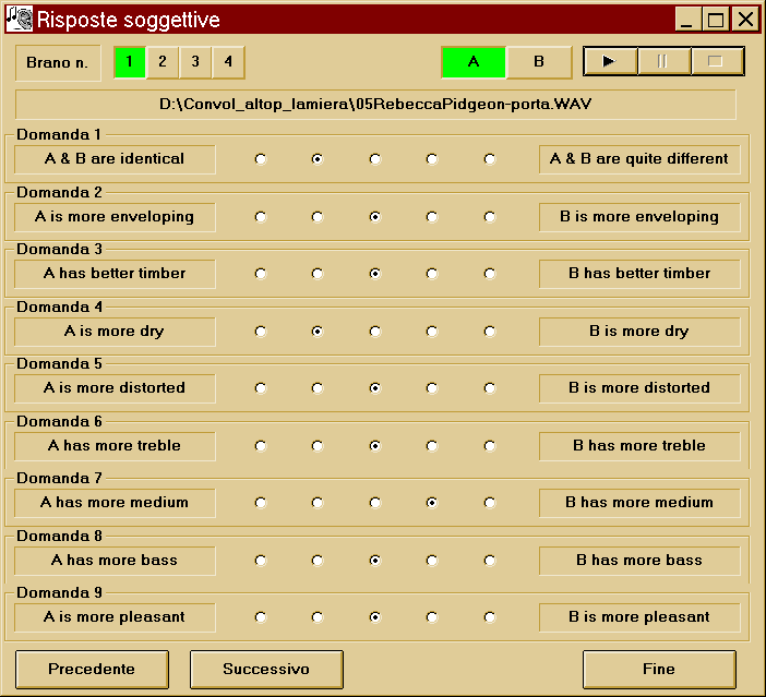
- A/B comparison
- Live recording & non-linear auralization
- 12 selected subjects
- 4 music samples
- 9 questions
- 5-dots horizontal scale
- Simple statistical analysis of the results
- A was the live recording, B was the auralization, but the listener did
not know this
|
|
35
|
- Statistical parameters – more advanced statistical methods would be
advisable for getting more significant results
|
|
36
|
- In the “IR switching” techniqque it is posssible to obtain some “memory
effect” employing a fast block convolution algorithm, instead of
processing “sample by sample”.
- The choice of the lenght of the processing block has to correspond to
the latency to level variations of the not-time-invariant device
|
|
37
|
- In the “diagonal volterra kernels” method, some meory effect can be
obtained adding a variable gain control droven by a time averaging block
- Also in this case, the choice of the time constant of the averaging
block needs to be aligned with the latency to level variations of the
not-time-invariant device
|

 Notes
Notes