1	Advanced beamforming techniques with microphone arrays A. Farina, S. Fontana, P. Martignon, A. Capra, C. Chiari Industrial Engineering Dept., University of Parma, Italy
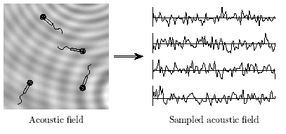
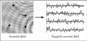
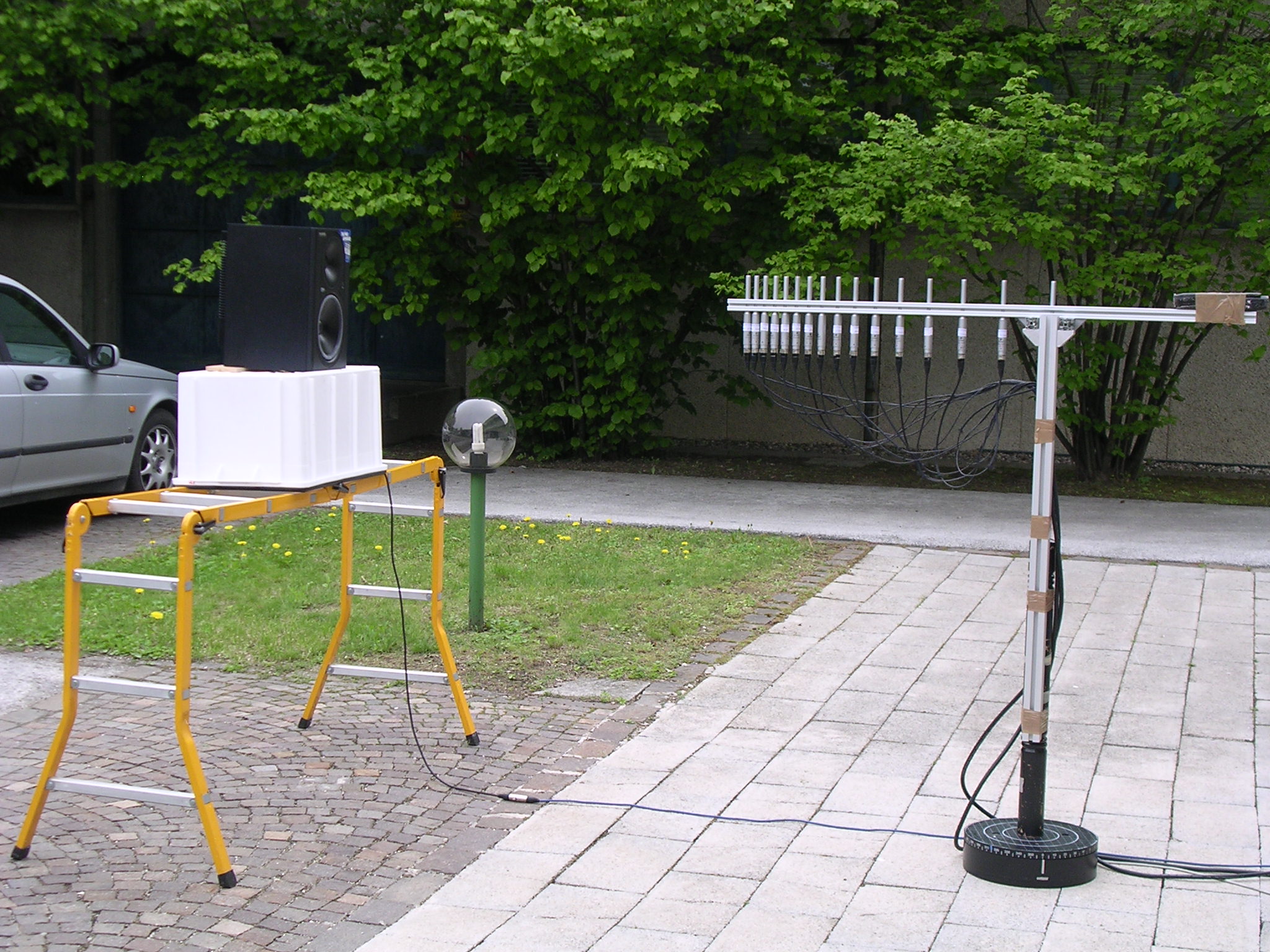
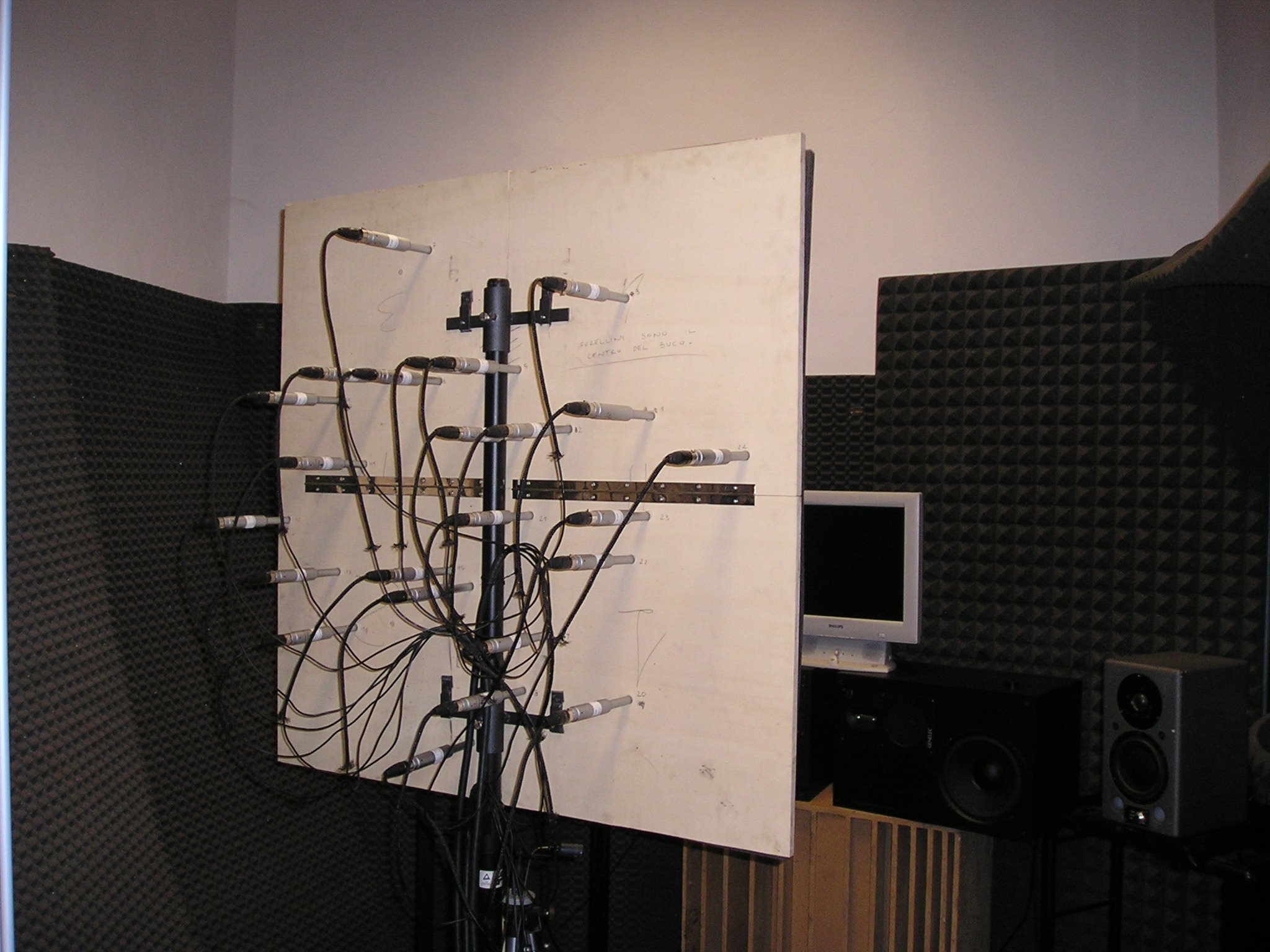
2	General Approach Whatever theory or method is chosen, we always start with N microphones, providing N signals x_i, and we derive from them M signals y_j And, in any case, each of these M outputs can be expressed by:
3	Microphone arrays: target, processing
4	Traditional approaches The processing filters h_ij are usually computed following one of several, complex mathematical theories, based on the solution of the wave equation (often under certaing simplifications), and assuming that the microphones are ideal and identical In some implementations, the signal of each microphone is processed through a digital filter for compensating its deviation, at the expense of heavier computational load
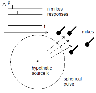
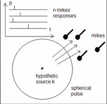
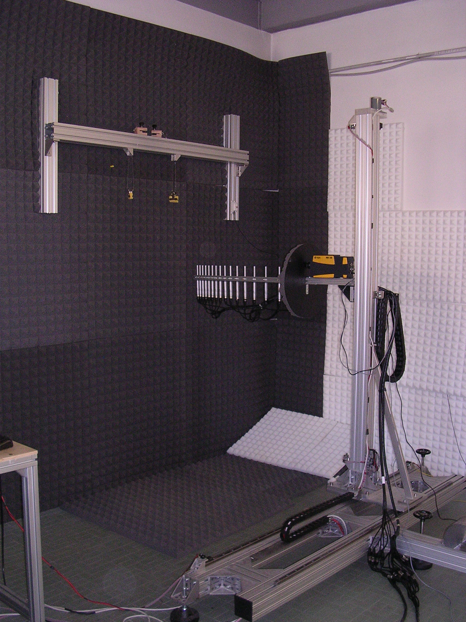
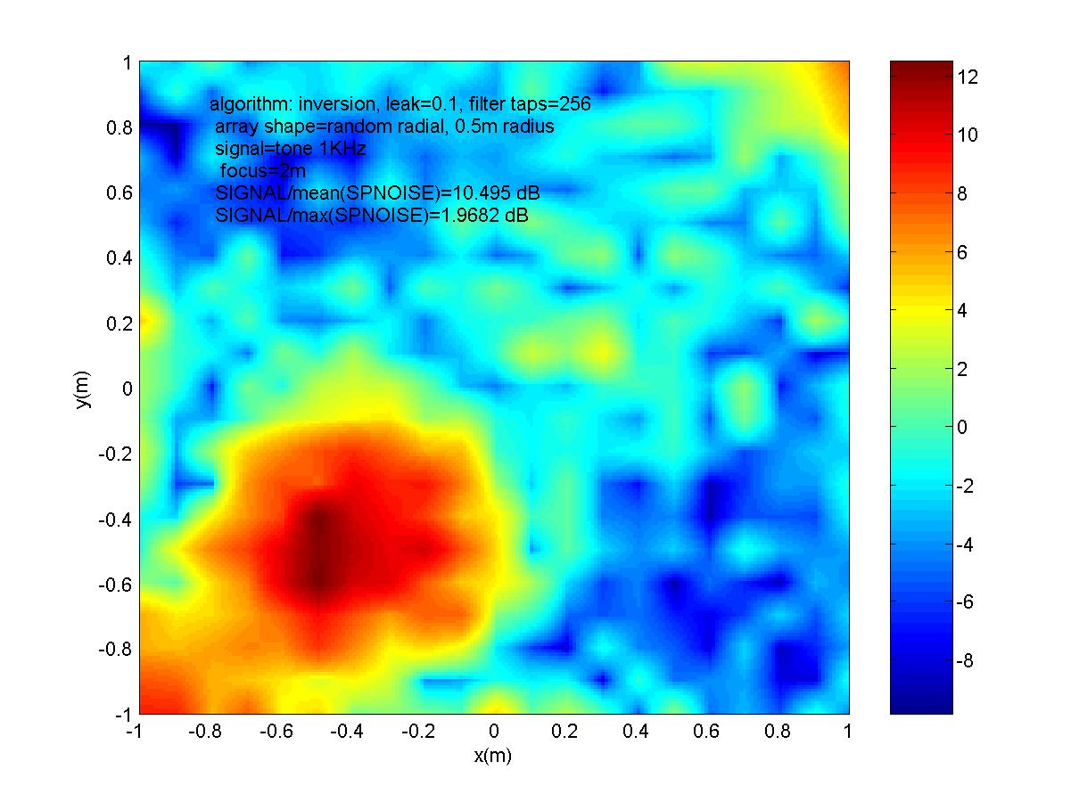
5	Novel approach No theory is assumed: the set of h_ij filters are derived directly from a set of impulse response measurements, designed according to a least-squares principle. In practice, a matrix of filtering coefficients, is formed, and the matrix has to be numerically inverted (usually employing some regularization technique). This way, the outputs of the microphone array are maximally close to the ideal responses prescribed This method also inherently corrects for transducer deviations and acoustical artifacts (shielding, diffractions, reflections, etc.)
6	Example: focusing a point source
7	Example: focusing a point source
8	Example: focusing a point source
9	System’s least-squares inversion For computing the matrix of N filtering coefficients h_ik, a least-squares method is employed. A “total squared error” e_tot is defined as:
10	Kirkeby’s regularization During the computation of the inverse filter, usually operated in the frequency domain, one usually finds expressions requiring to compute a ratio between complex spectra (H=A/D). Computing the reciprocal of the denominator D is generally not trivial, as the inverse of a complex, mixed-phase signal is generally unstable. The Nelson/Kirkeby regularization method is usually employed for this task:
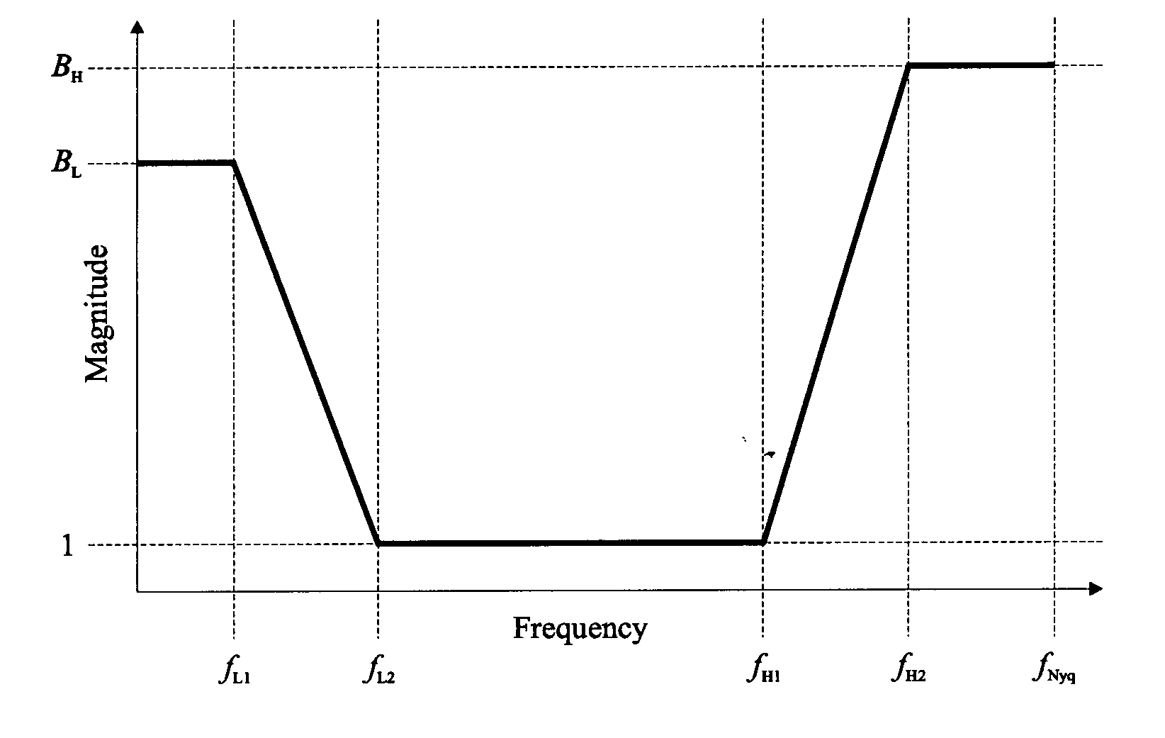
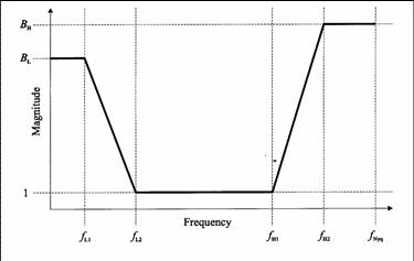
11	Spectral shape of the regularization parameter e(w) At very low and very high frequencies it is advisable to increase the value of e.
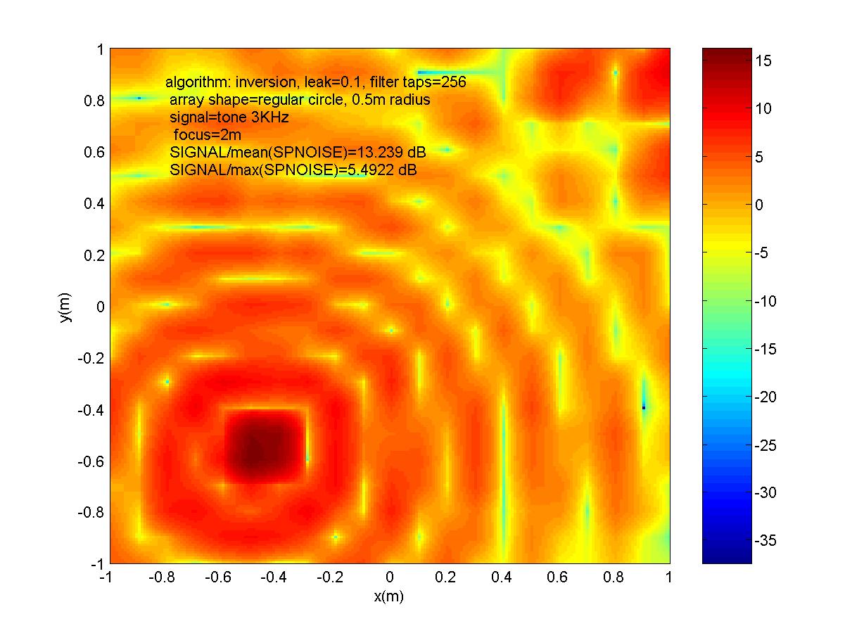
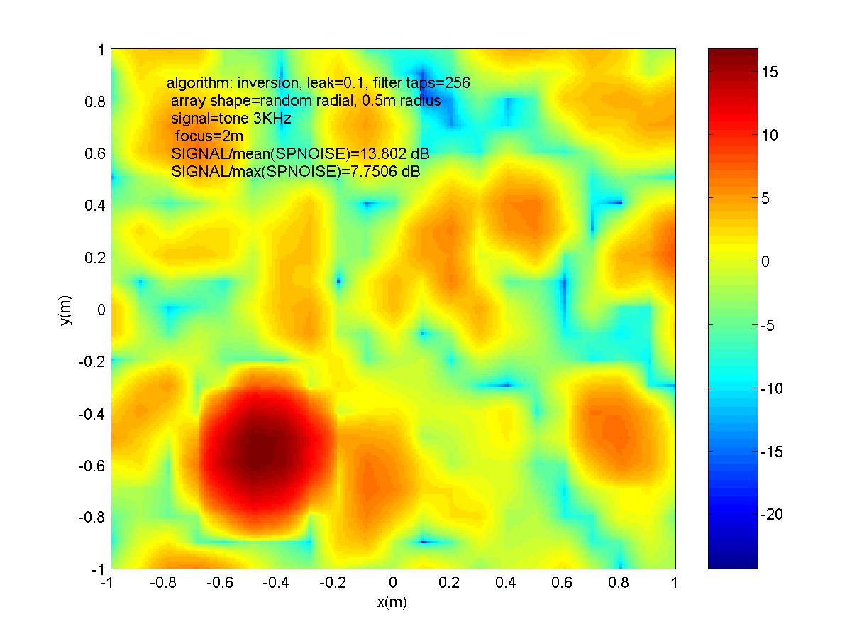
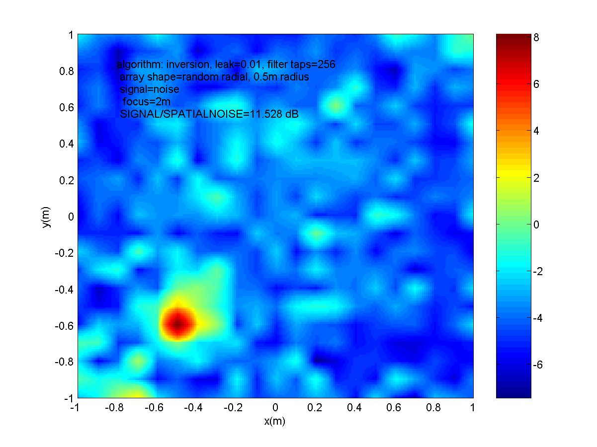
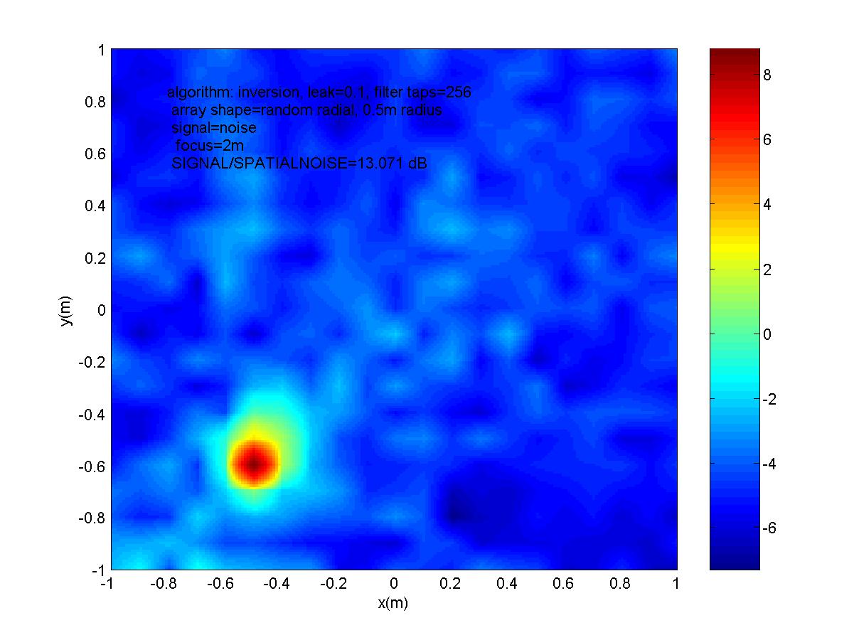
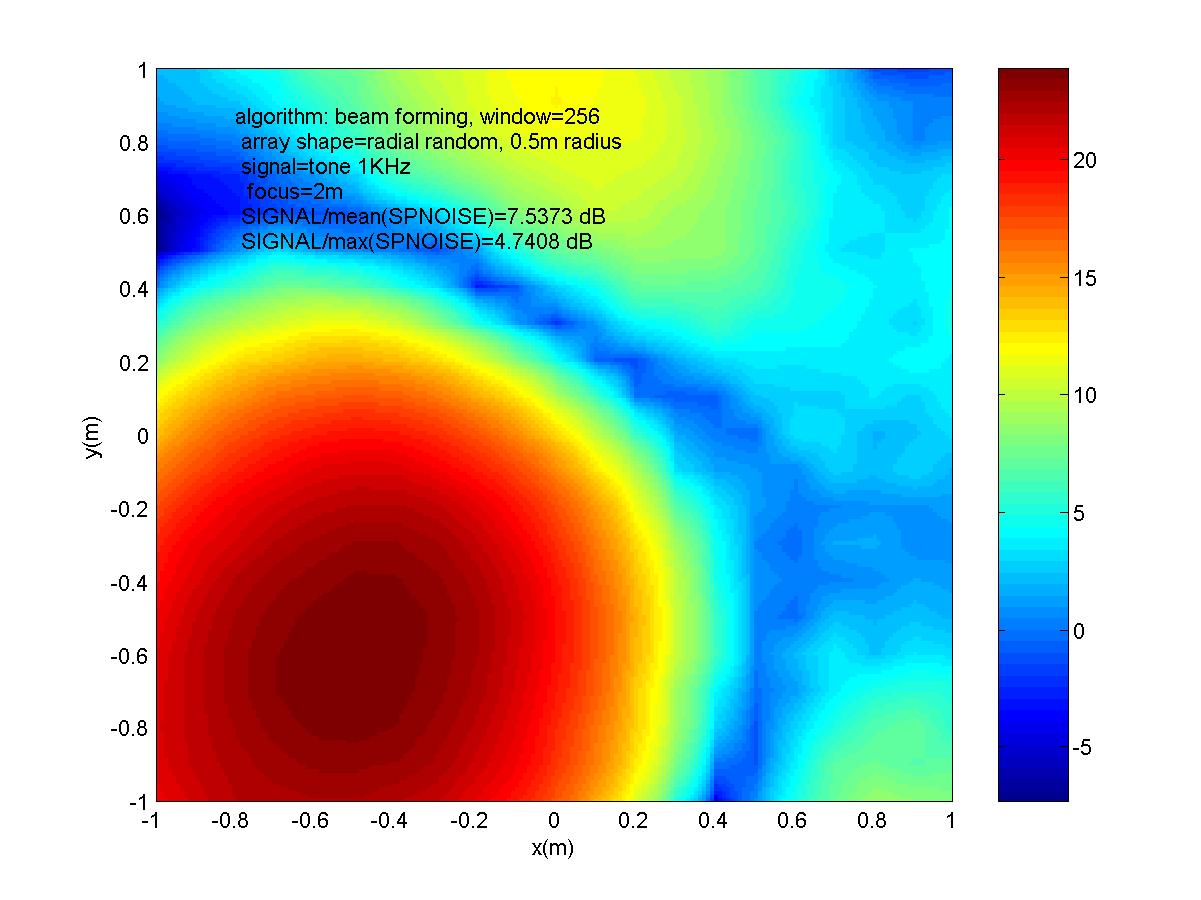
12	Critical aspects LOW frequencies: wavelength longer than array width - no phase difference between mikes - local approach provide low spatial resolution (single, large lobe) - global approach simply fails (the linear system becomes singular) MID frequencies: wavelength comparable with array width -with local approach secondary lobes arise in spherical or plane wave detection (negligible if the total bandwidth is sufficiently wide) - the global approach works fine, suppressing the side lobes, and providing a narrow spot. HIGH frequencies: wavelength is shorter than twice the average mike spacing (Nyquist limit) - spatial undersampling - spatial aliasing effects – random disposition of microphones can help the local approach to still provide some meaningful result - the global approach fails again
13	Linear array
14	Linear array - calibration
15	Linear array - polar plots
16	Linear array - practical usage
17	Linear array - practical usage
18	Linear array - test results (small loudspeaker)
19	Linear array - test results (rectangular wood panel)
20	Planar array (“acoustic camera”)
21	Random array vs. Circular array
22	Circular array vs. Random array
23	Beamforming vs. Inverse filters
24	Effect of the regularization parameter
25	Indoor application (source localisation)
26	Outdoor application
27	Real time processing: work on progress
28	“X-volver” VST plugin
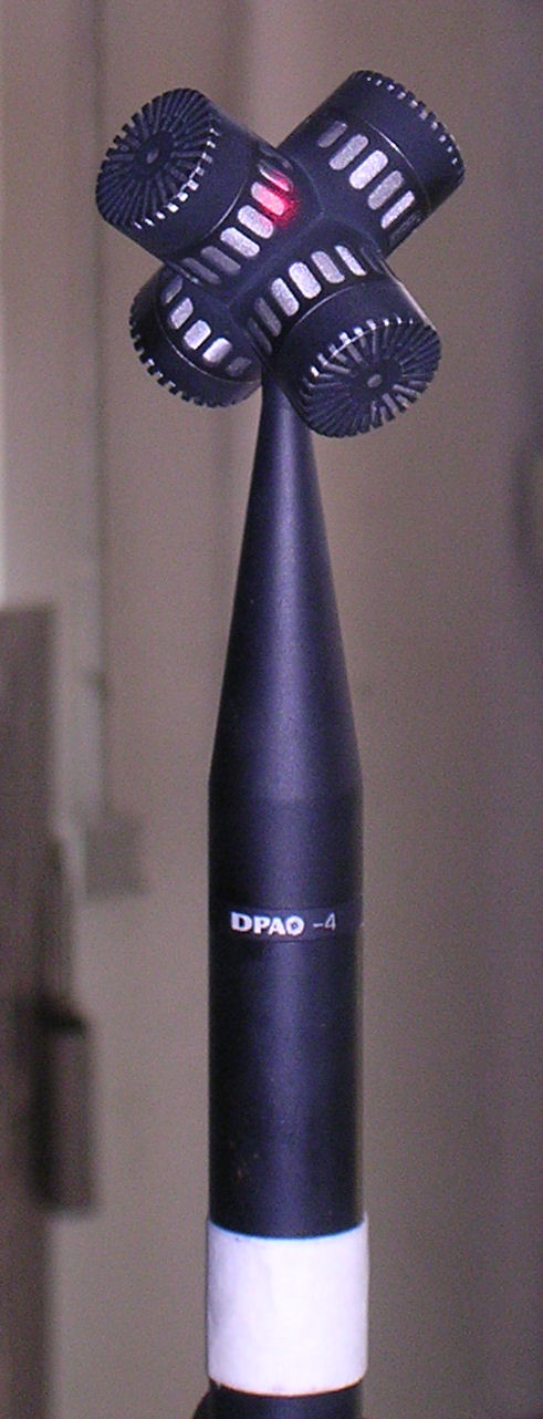
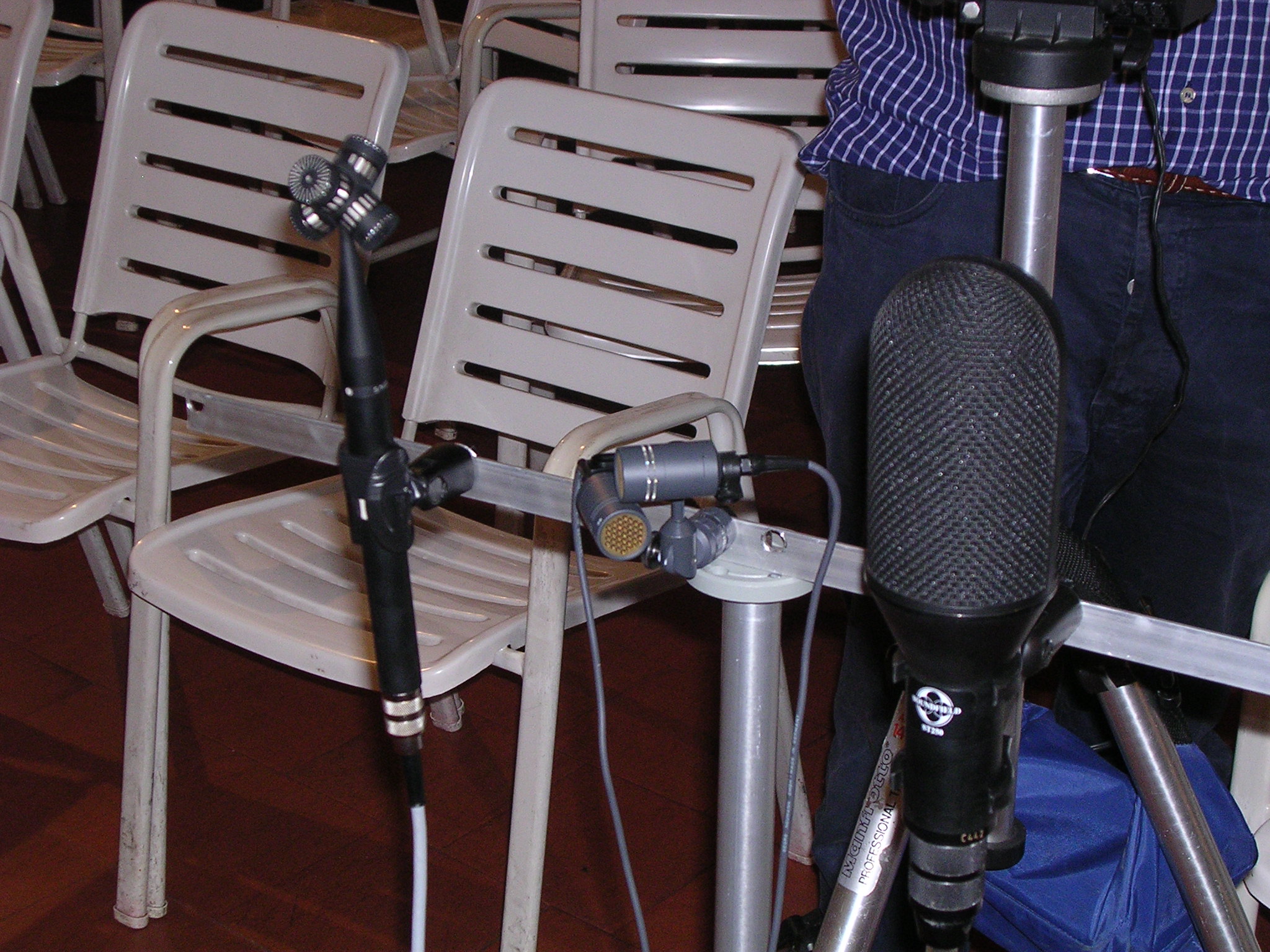
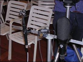
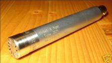
29	3D arrays DPA-4 A-format microphone 4 closely-spaced cardioids A set of 4x4 filters is required for getting B-format signals Global approach for minimizing errors over the whole sphere
30	IR measurements on the DPA-4
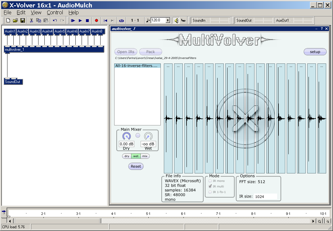
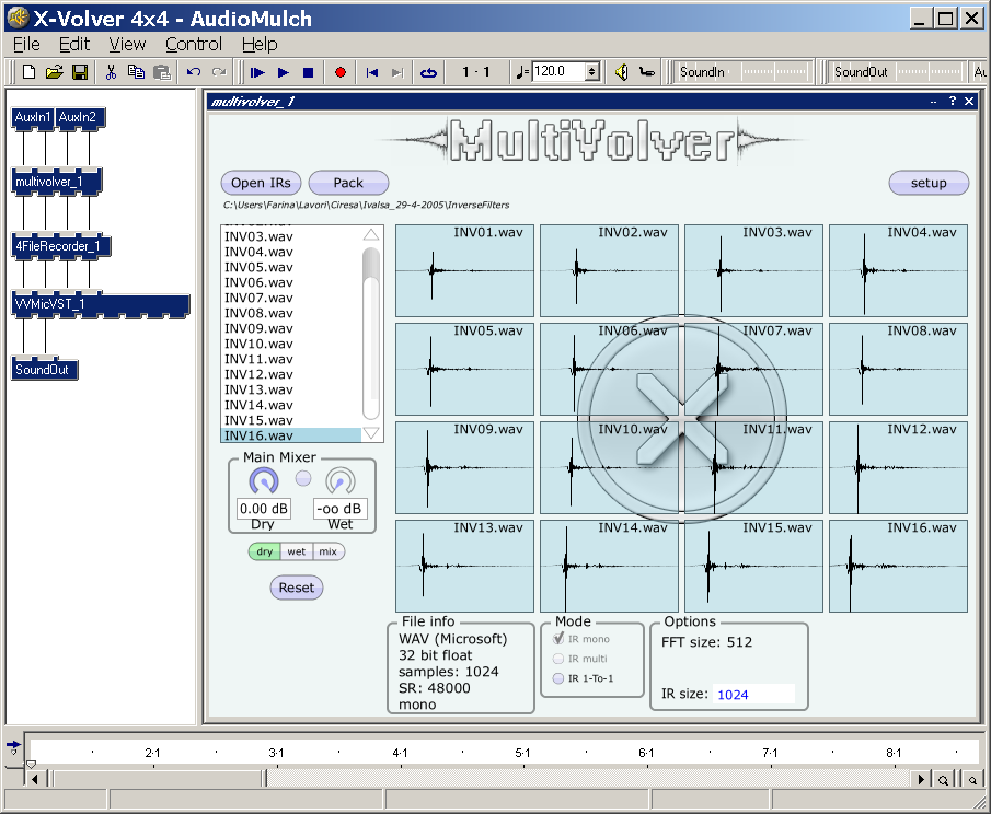
31	Computation of the inverse filters A set of 16 inverse filters is required (4 inputs, 4 outputs) For any of the 84 measured directions, a theoretical response can be computed for each of the 4 output channels (W,X,Y,Z) So 84x4=336 conditions can be set:
32	Real-time implementation
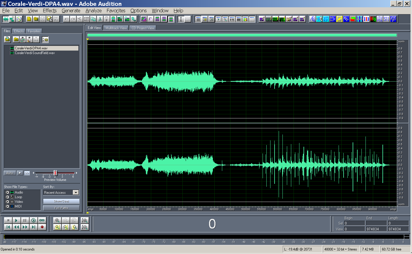
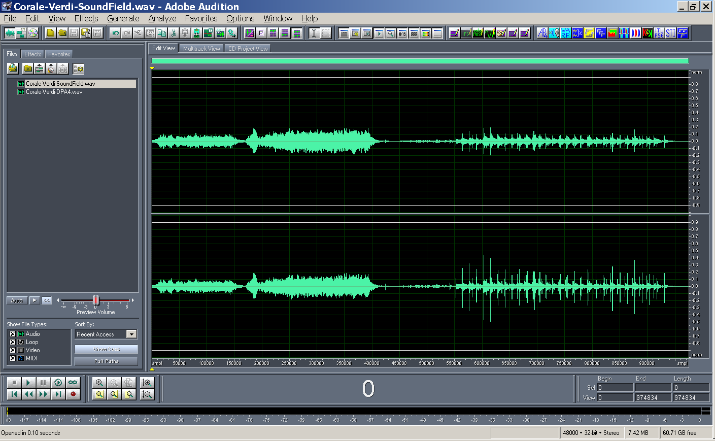
33	Microphone comparison 2 crossed Neumann K-140 were compared with a pair of virtual cardioids derived from B-format signals, recorded either with a Soundfield ST-250 and with the new DPA-4
34	Sound samples The new DPA-4 outperforms the Soundfield in terms of stereo separation and frequency response, and is indistinguishable from the “reference” Neumann cardioids
35	Conclusions The numerical approach to array processing does not require complex mathematical theories The quality of the processing FIR filters depends strongly on the quality of the impulse response measurements The method allows for the usage of imperfect arrays, with low-quality transducers and irregular geometry A new fast convolver has been developed for real-time applications
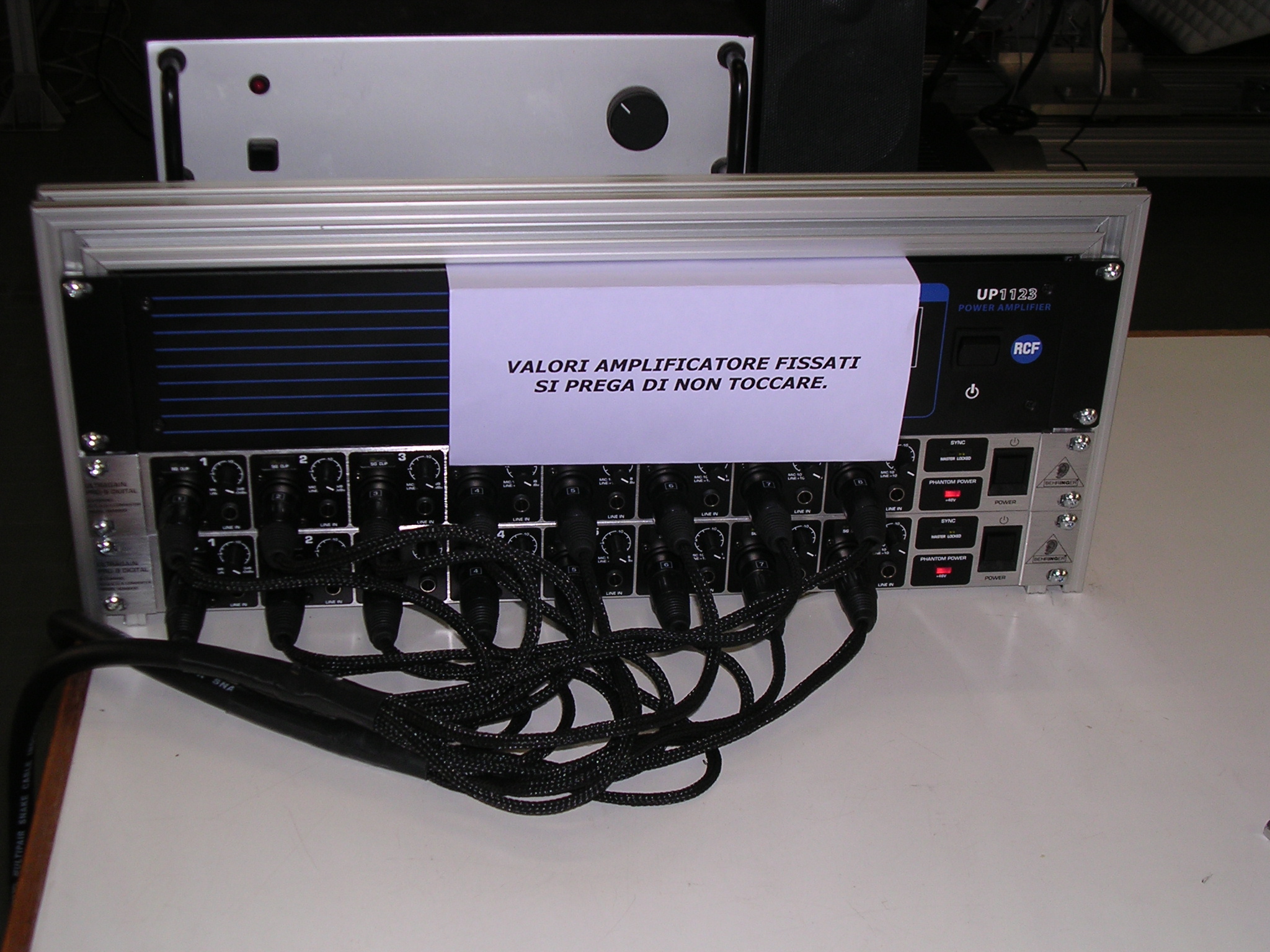
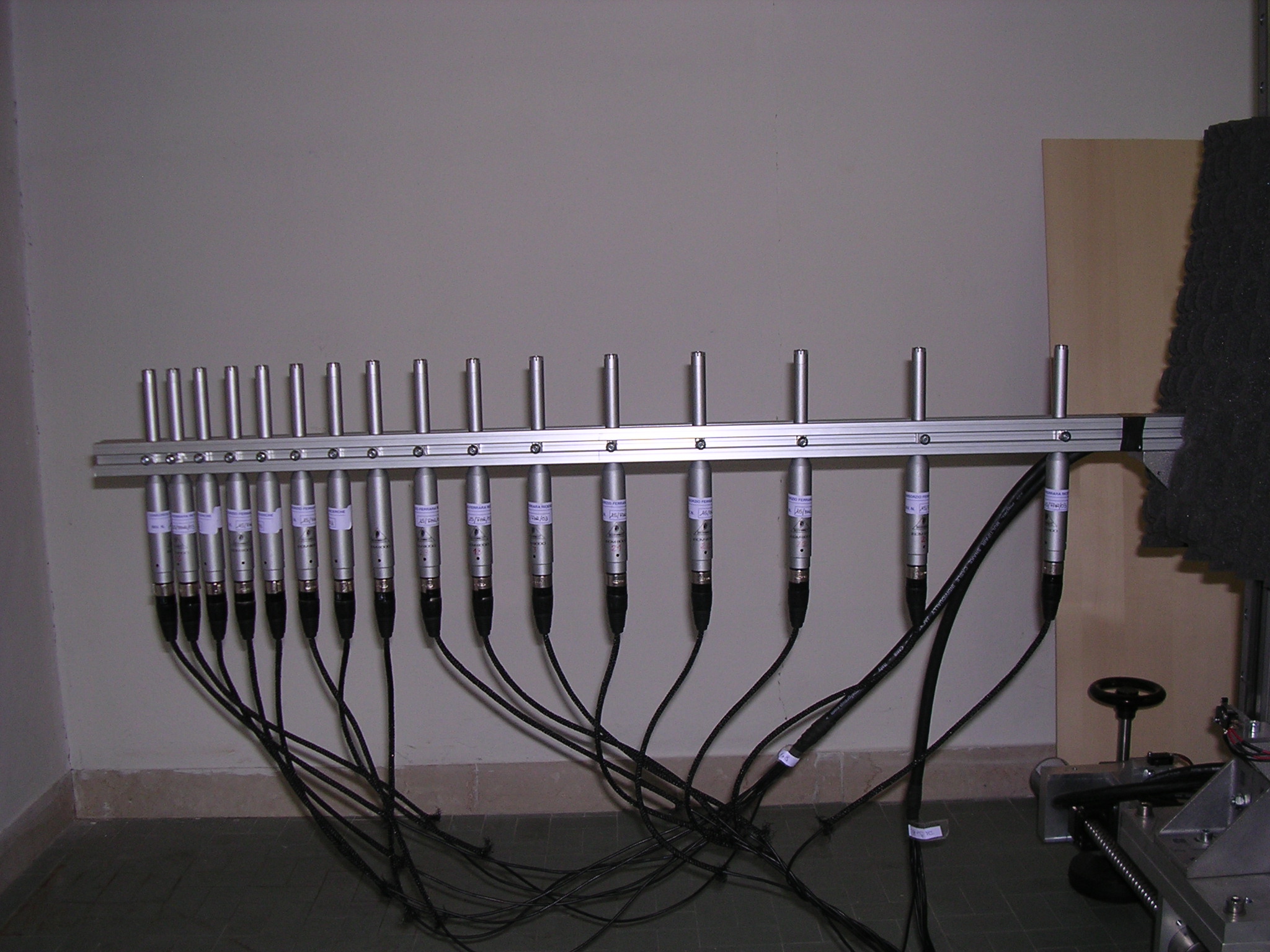
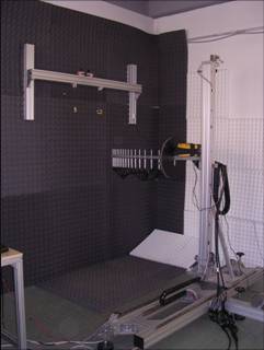
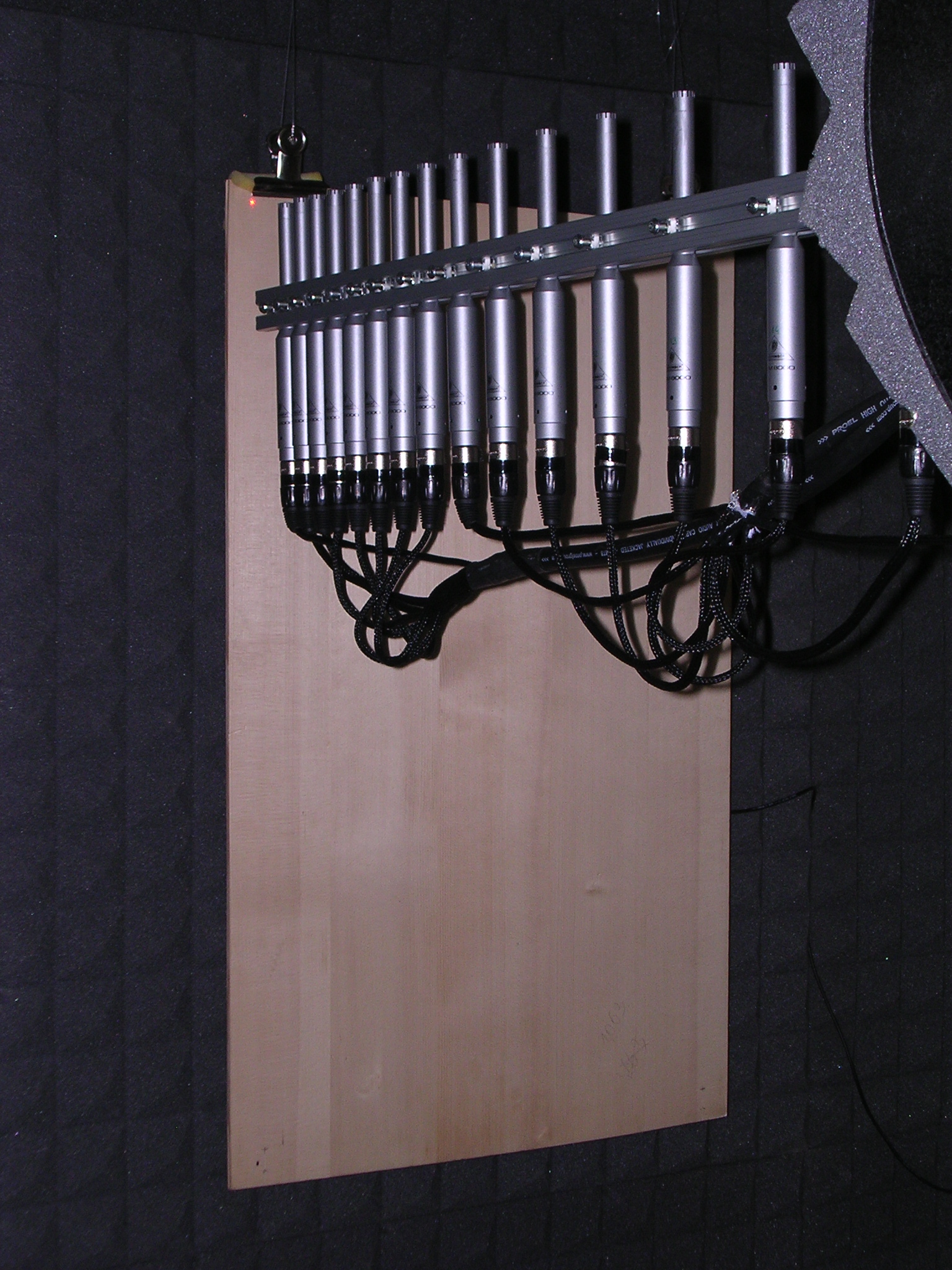
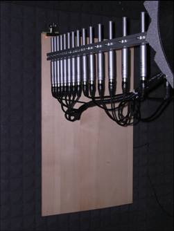
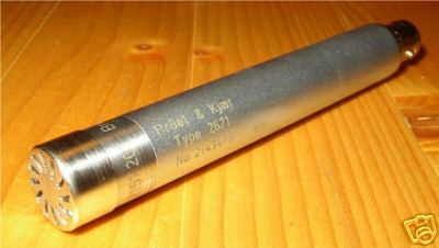
36	Future developements A new 24-microphones array is being assembled, employing 24 high quality B&K 4188 microphones
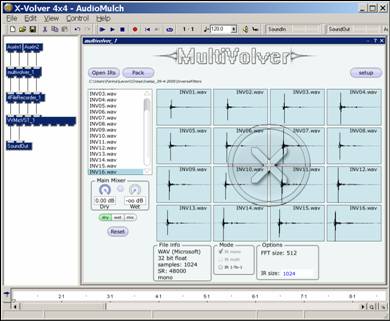
37	Future developements The Multivolver VST plugin will be improved (Intel IPP 5.0 FFT subroutines, multithread, rebuffering for employing larger FFT blocks even when the host block is limited) Fast switching of the set of impulse responses will be added, with MIDI control of the running set (for head-tracking, or realtime spatialisation simulating movement of sources or receivers) A new standalone program will be developed for speeding up the computation of the sets of inverse filters (the actual Matlab implementation is very slow and unfriendly)