1	HISTORY OF ROOM IMPULSE RESPONSE MEASUREMENTS
2	Time Line
3	Basic sound propagation scheme
4	The Past
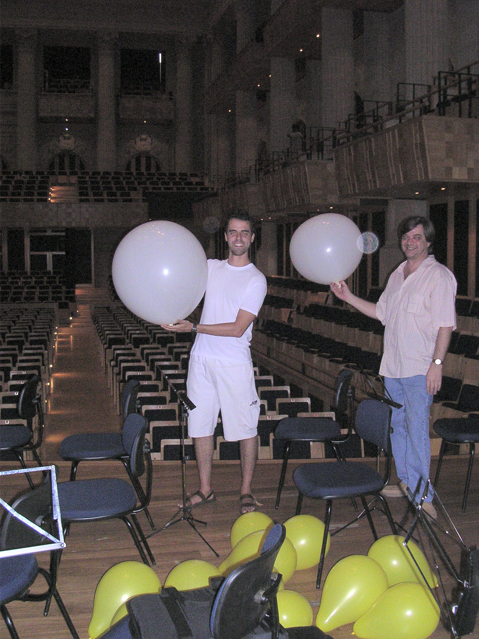
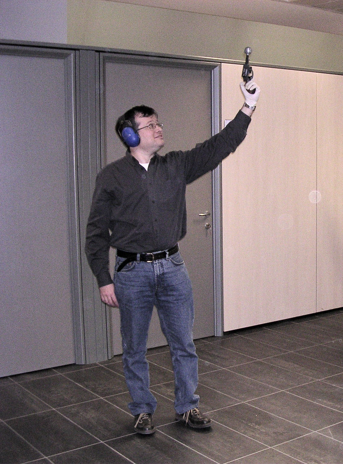
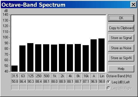
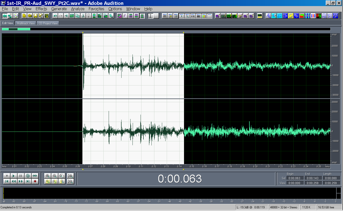
5	Traditional measurement methods Pulsive sources: ballons, blank pistol
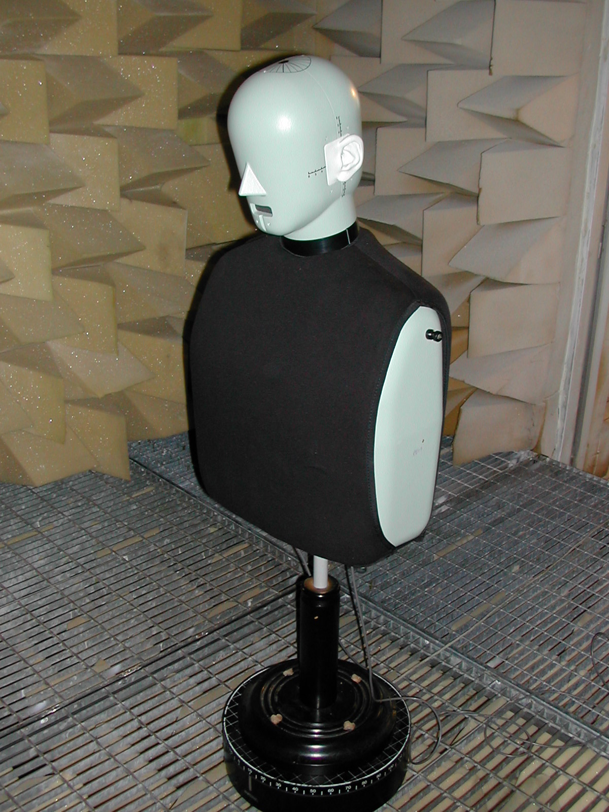
6	Example of a pulsive impulse response
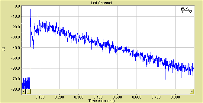
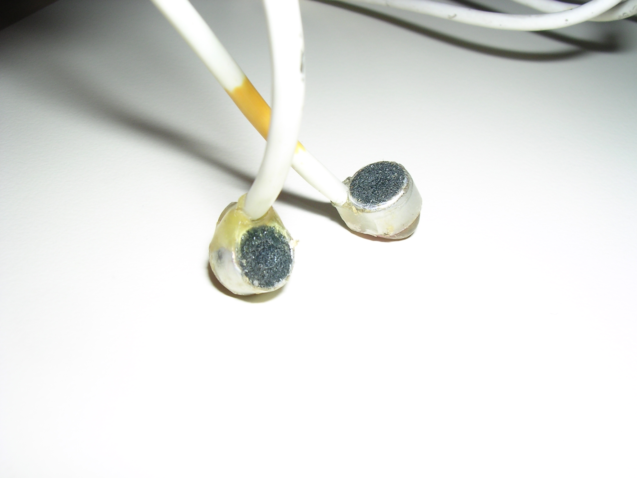
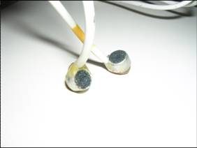
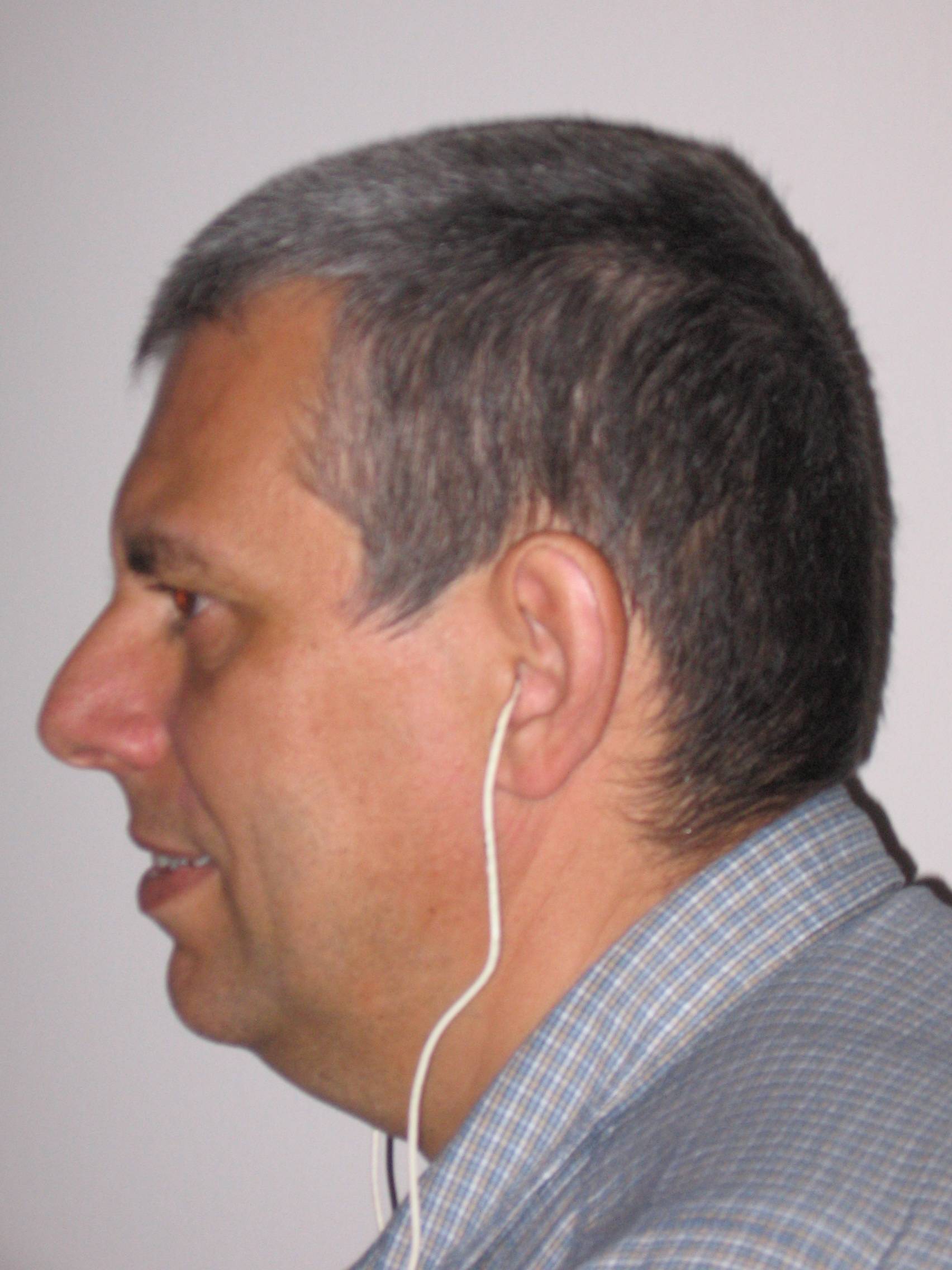
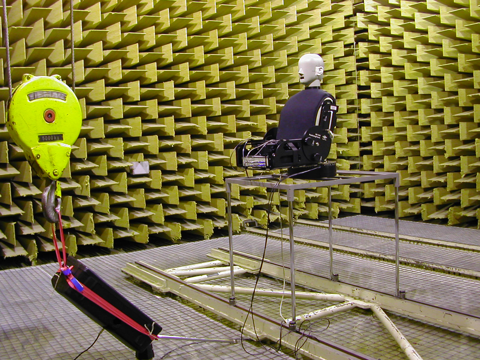
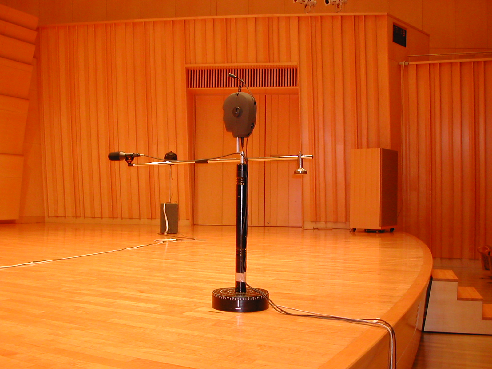
7	Test with binaural microphones Cheap electret mikes in the ear ducts
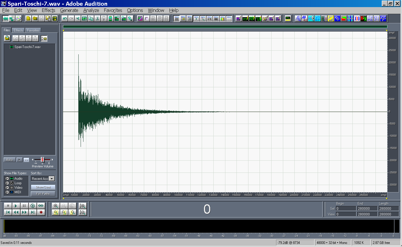
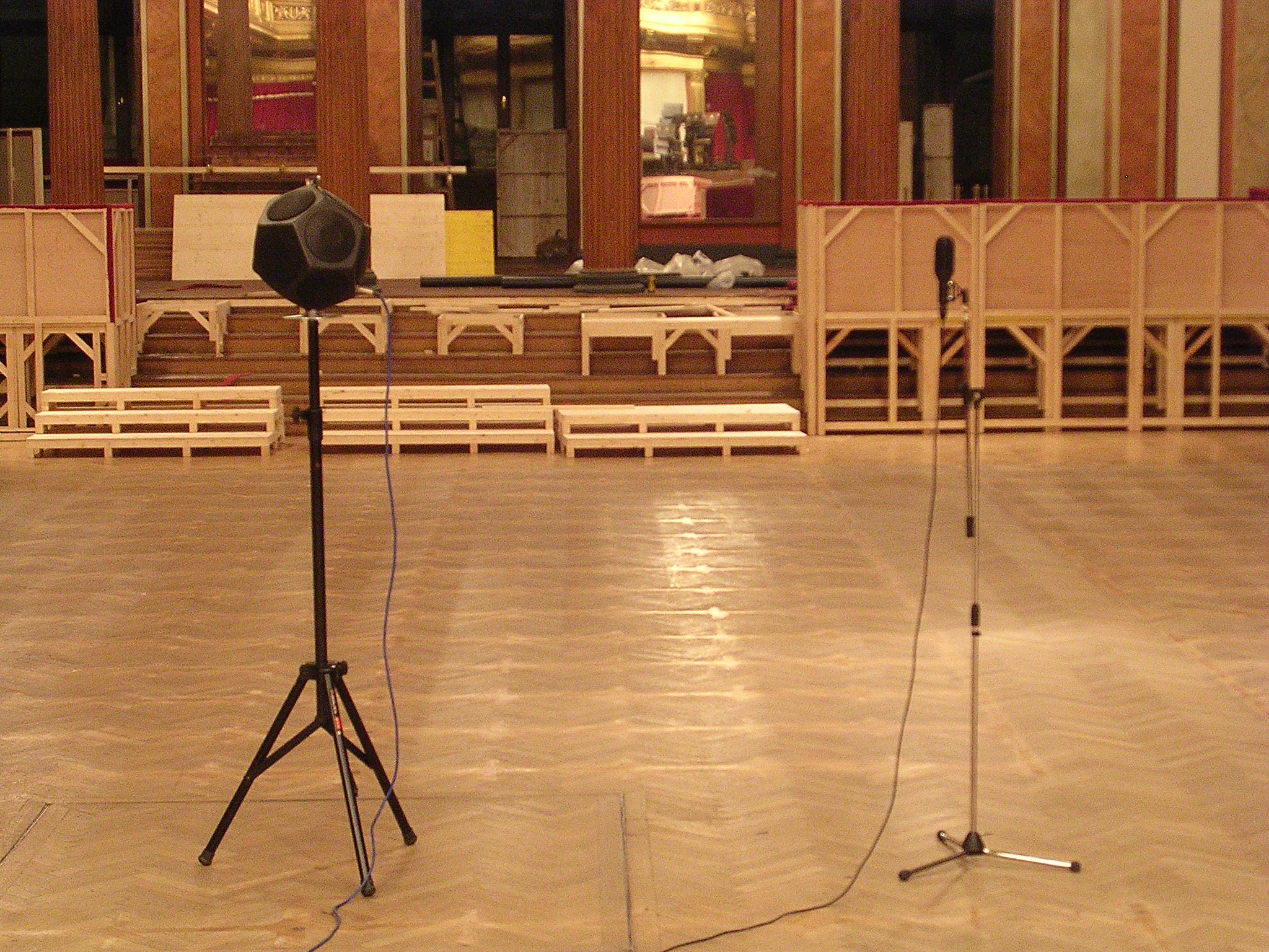
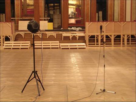
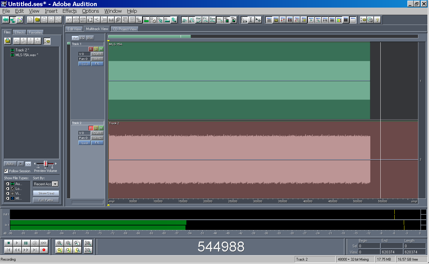
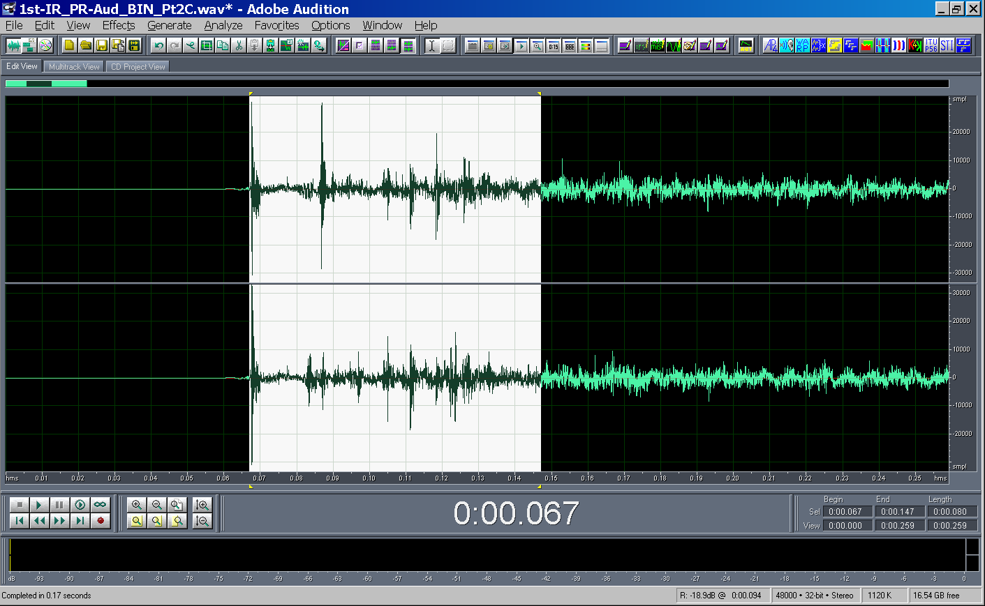
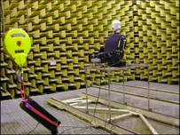
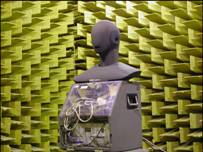
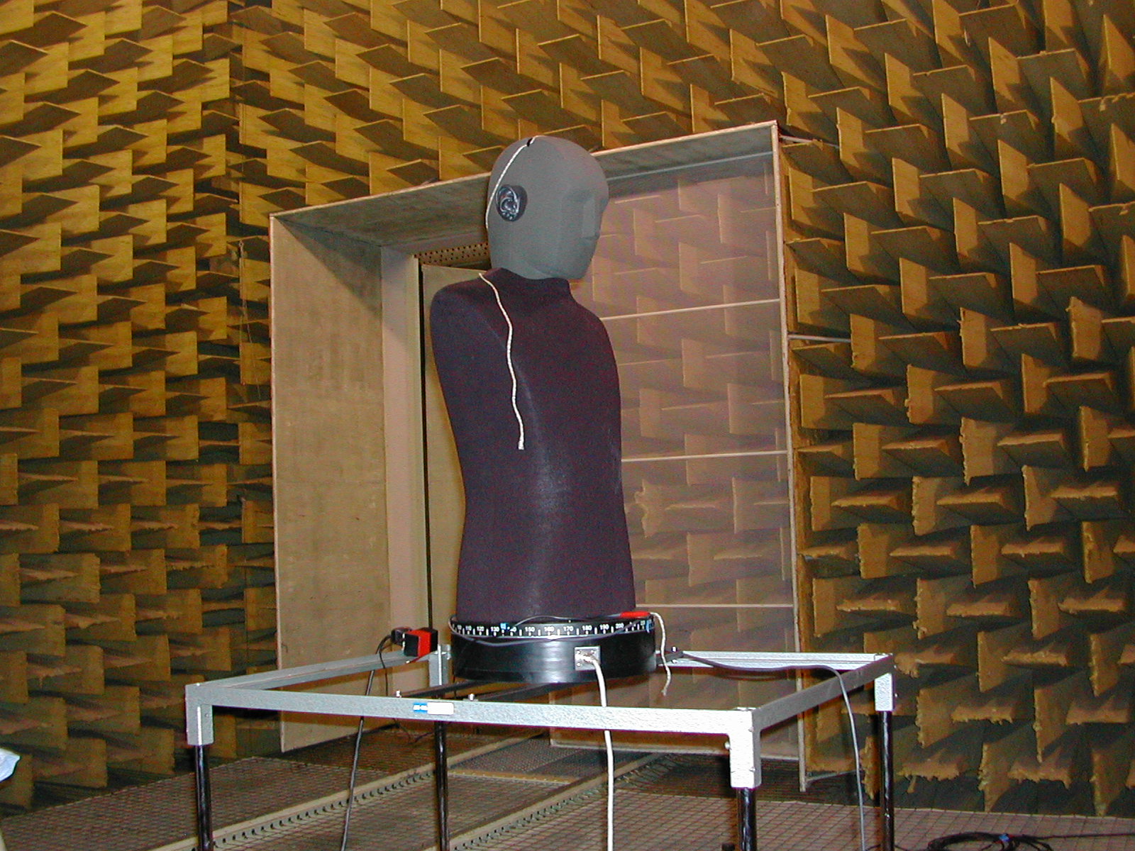
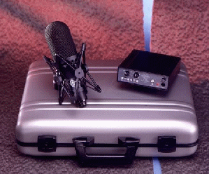
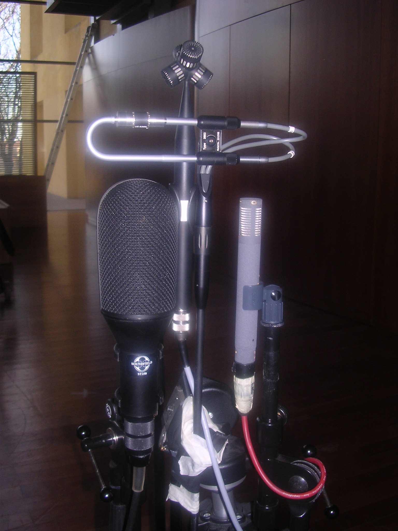
8	Loudspeaker as sound source A loudspeaker is fed with a special test signal x(t), while a microphone records the room response A proper deconvolution technique is required for retrieving the impulse response h(t) from the recorded signal y(t)
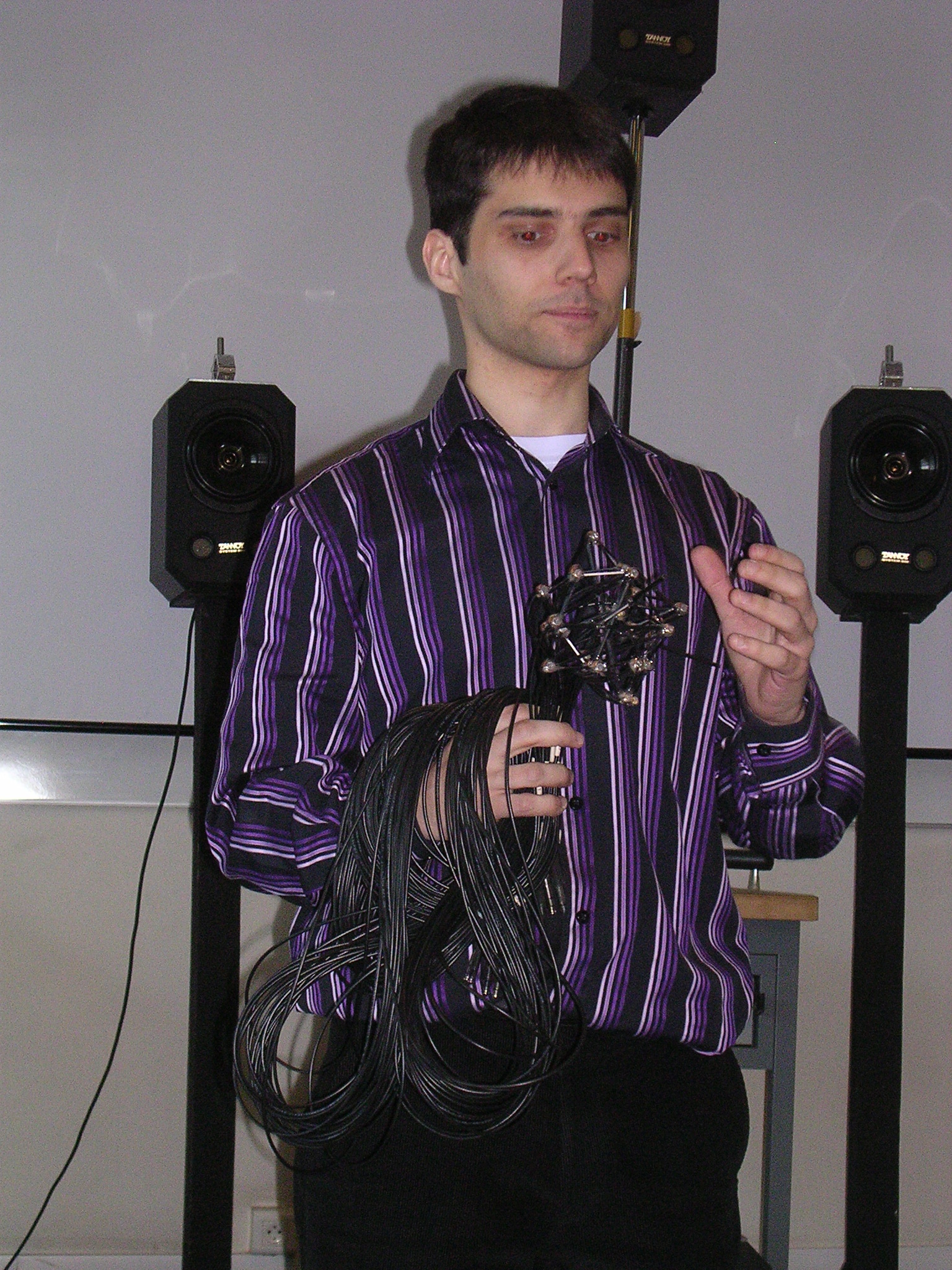
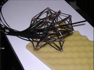
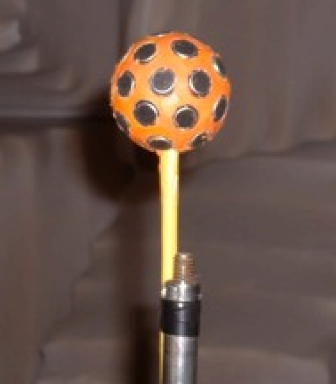
9	Measurement process The desidered result is the linear impulse response of the acoustic propagation h(t). It can be recovered by knowing the test signal x(t) and the measured system output y(t). It is necessary to exclude the effect of the not-linear part K and of the background noise n(t).
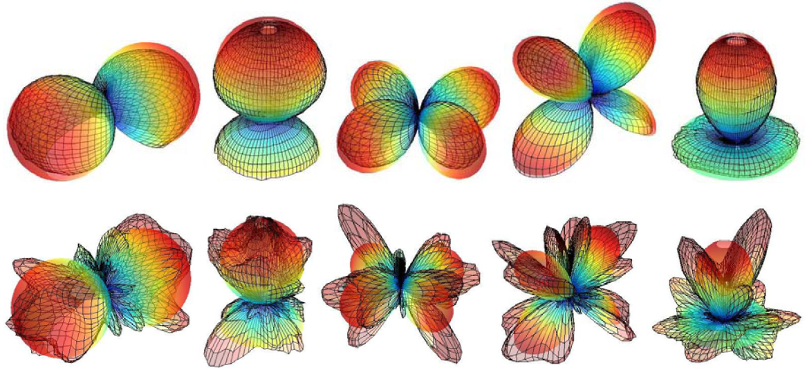
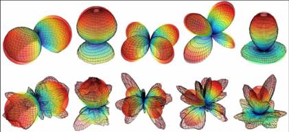
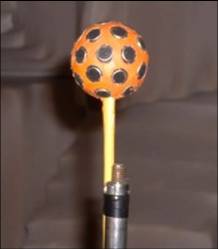
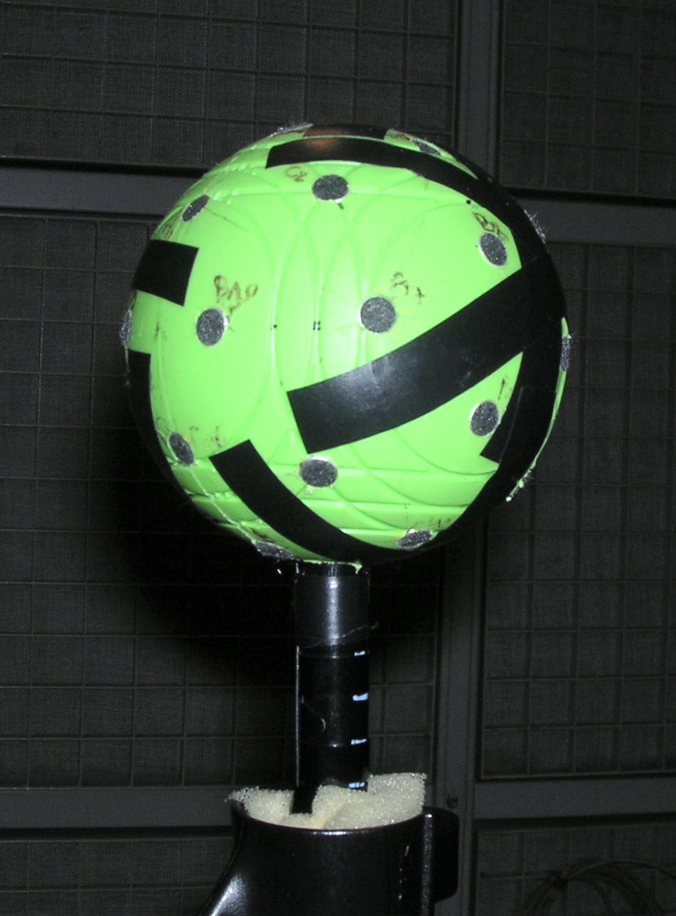
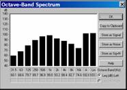
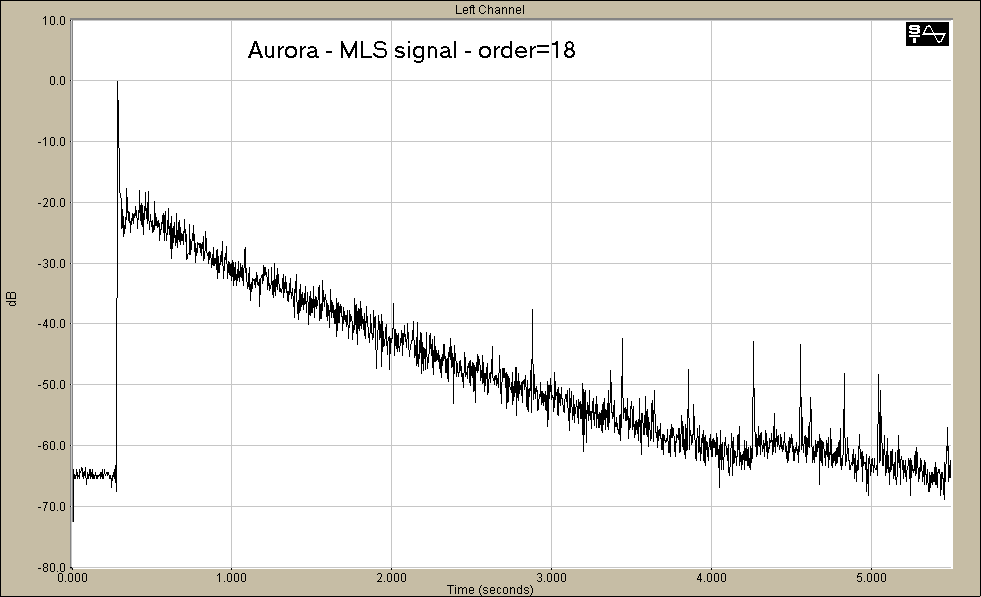
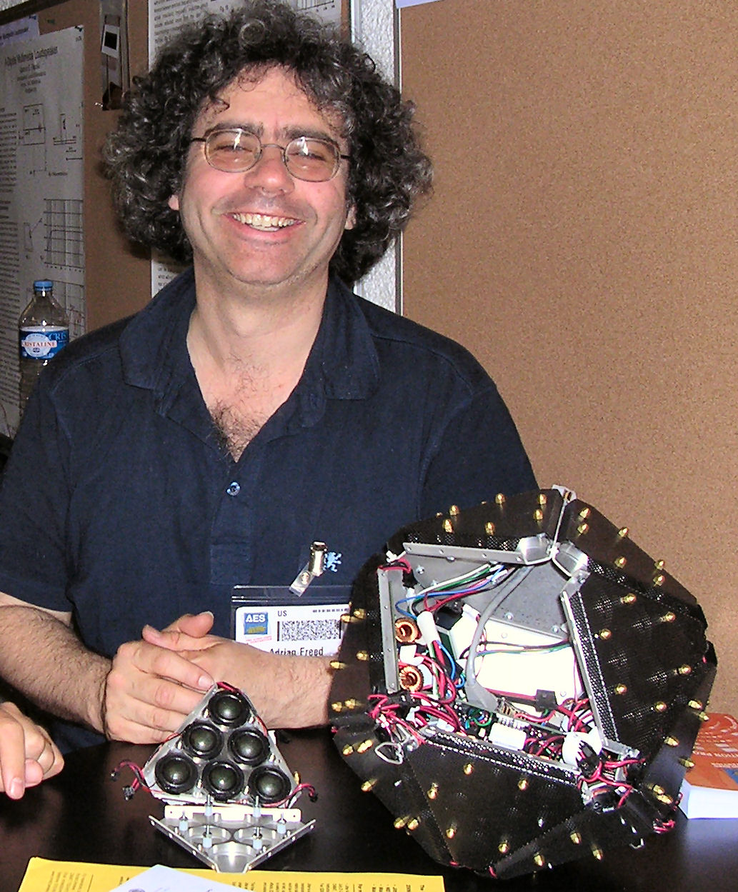
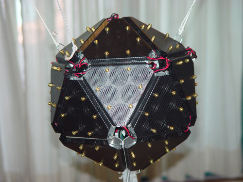
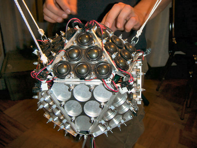
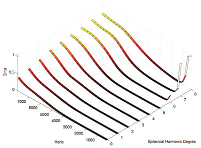
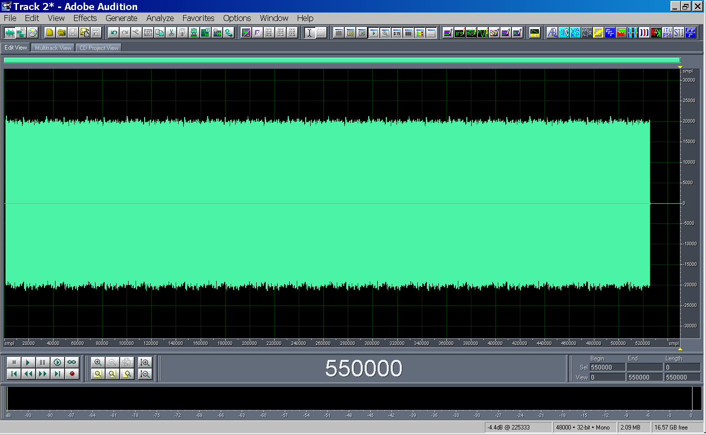
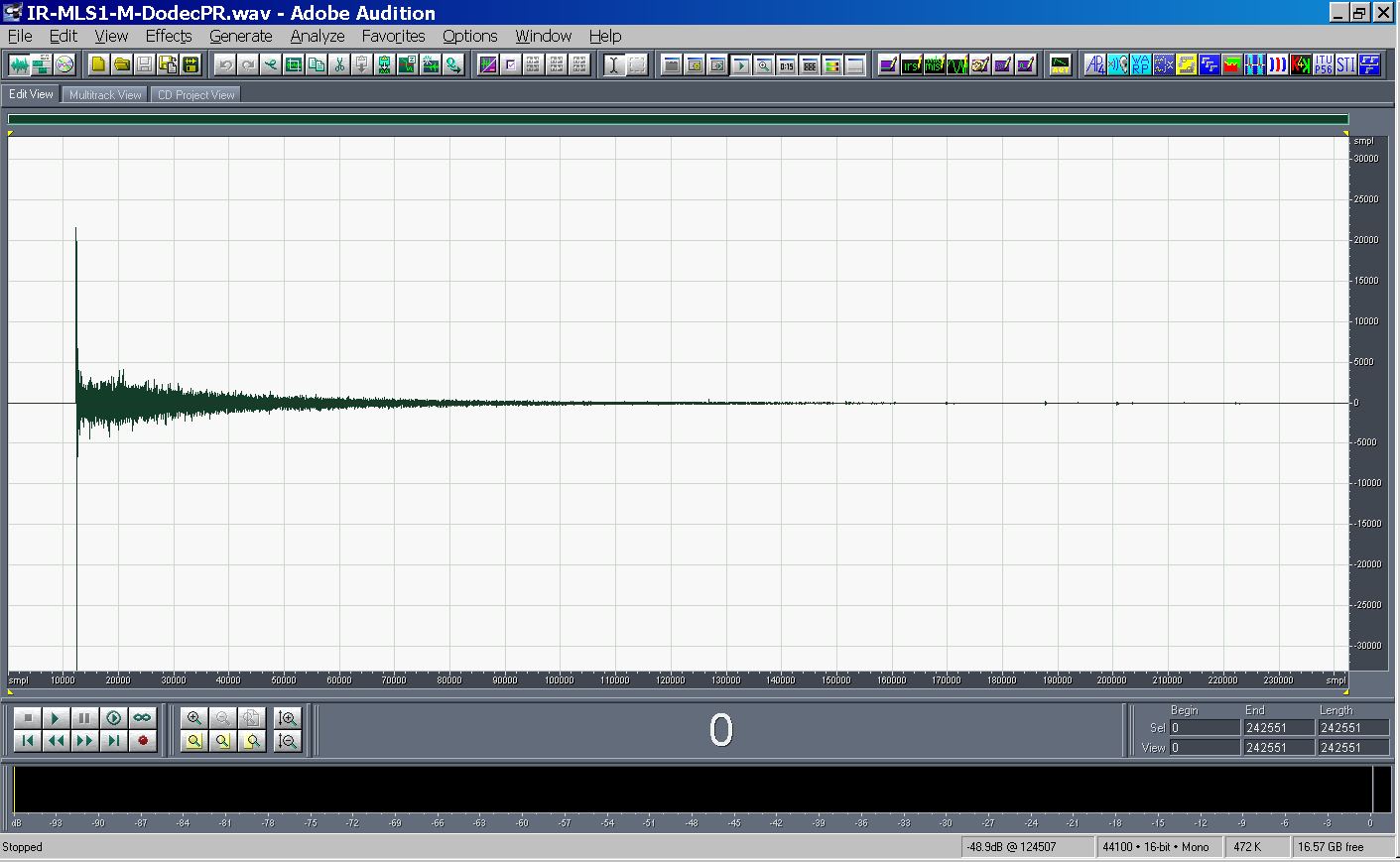
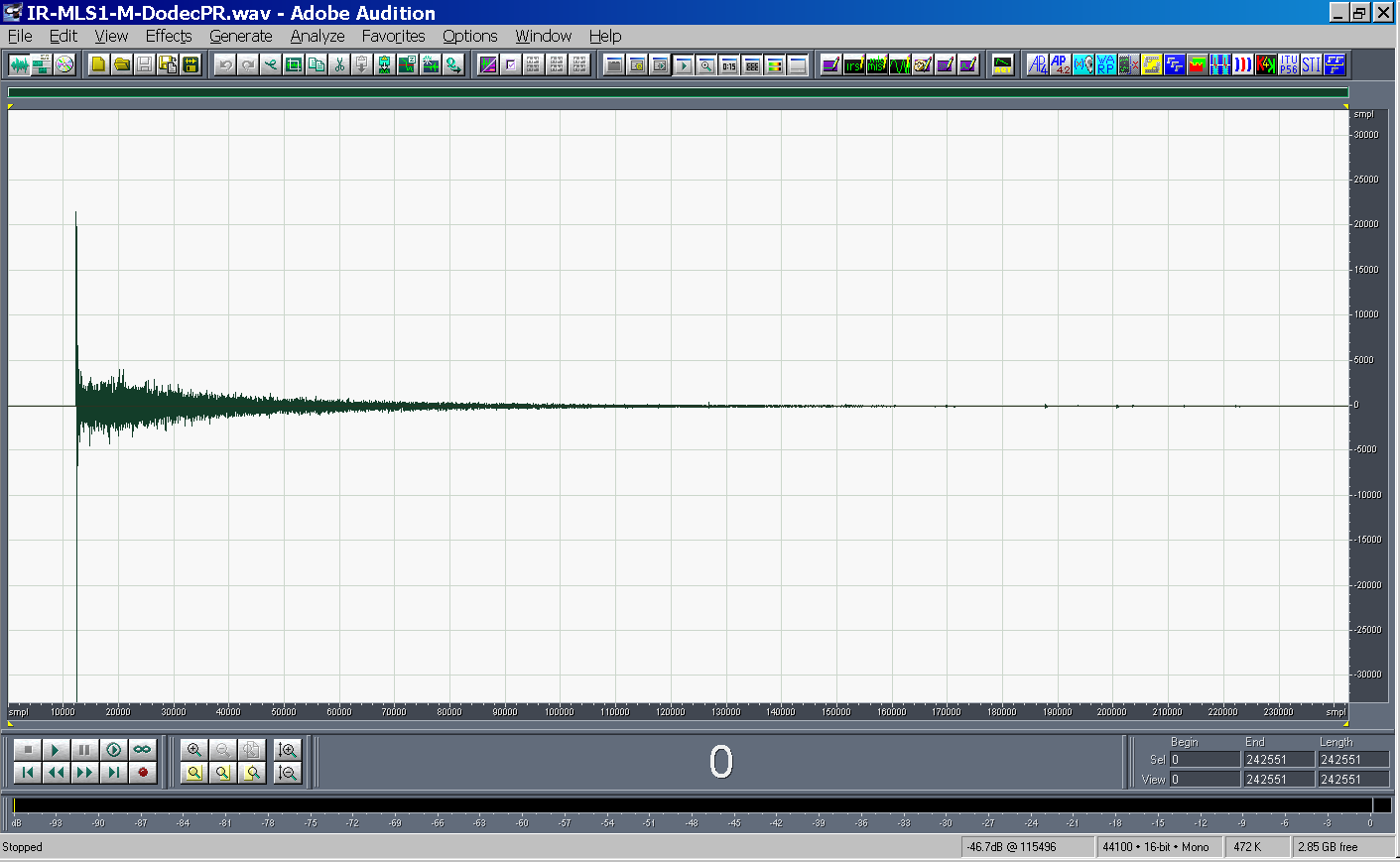
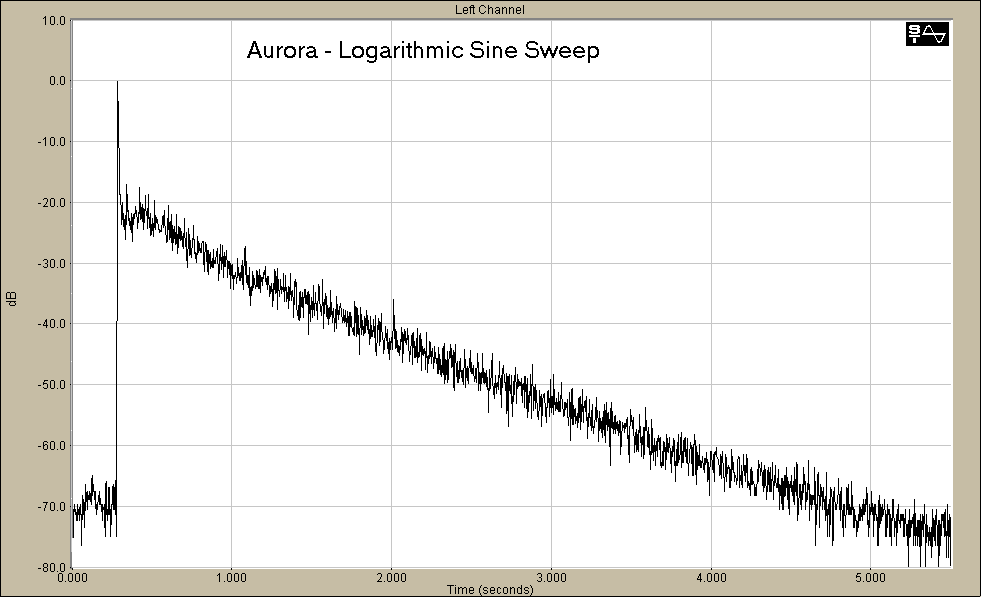
10	Electroacoustical methods Different types of test signals have been developed, providing good immunity to background noise and easy deconvolution of the impulse response: MLS (Maximum Lenght Sequence, pseudo-random white noise) TDS (Time Delay Spectrometry, which basically is simply a linear sine sweep, also known in Japan as “stretched pulse” and in Europe as “chirp”) ESS (Exponential Sine Sweep) Each of these test signals can be employed with different deconvolution techniques, resulting in a number of “different” measurement methods Due to theoretical and practical considerations, the preference is nowadays generally oriented for the usage of ESS with not-circular deconvolution
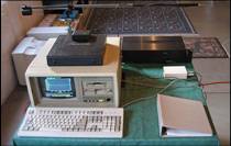
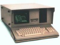
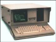
11	The first MLS apparatus - MLSSA MLSSA was the first apparatus for measuring impulse responses with MLS
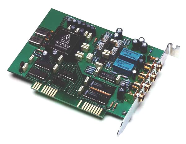
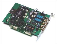
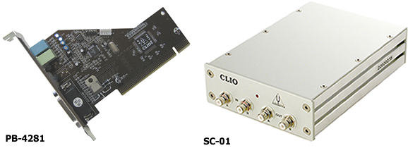
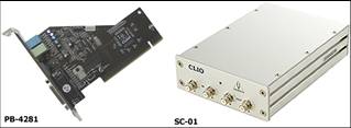
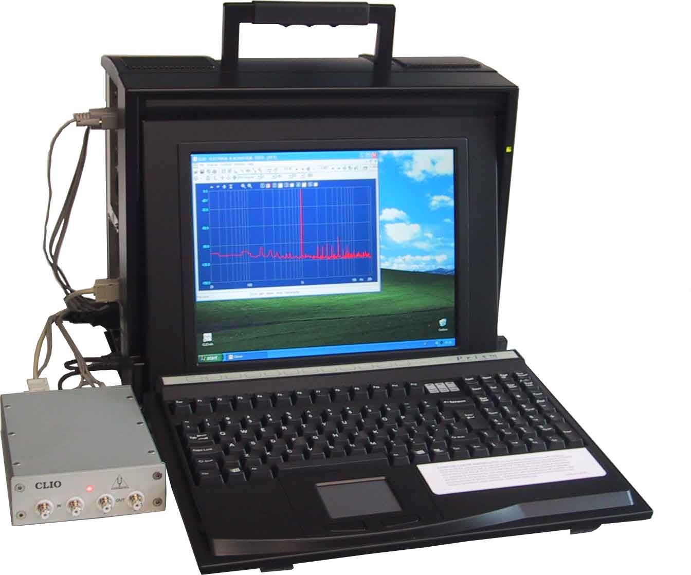
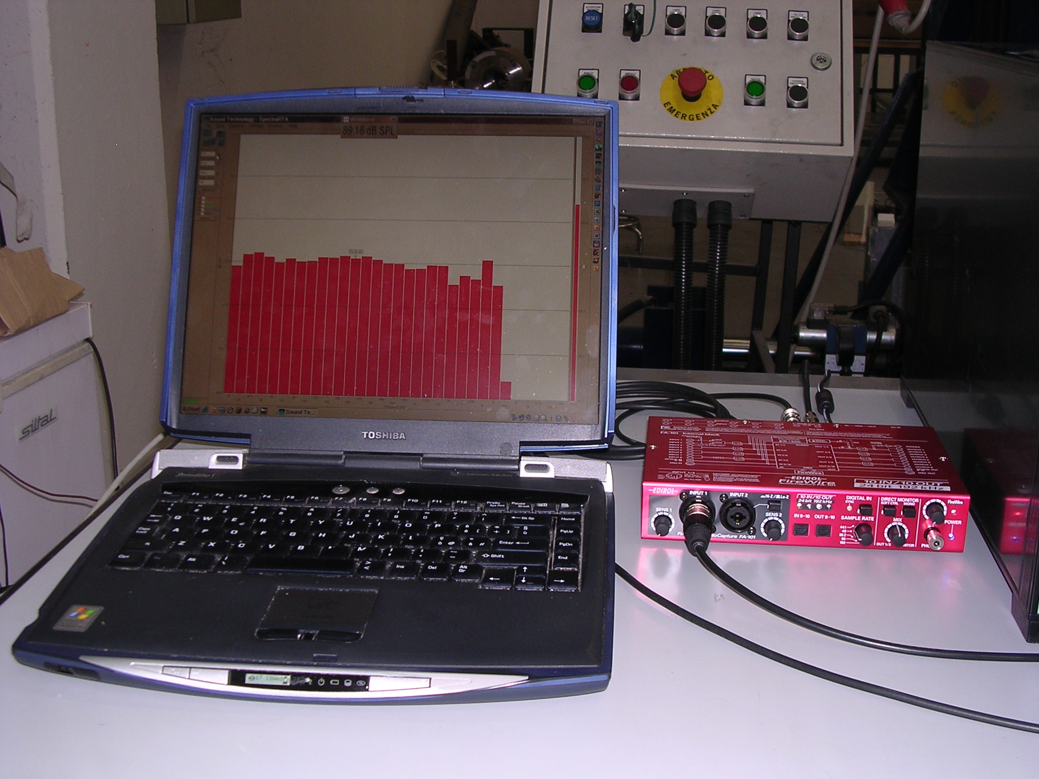
12	More recently - the CLIO system The Italian-made CLIO system has superseded MLSSA for most electroacoustics applications (measurement of loudspeakers, quality control)
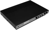
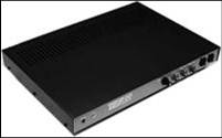
13	The first TDS apparatus - TEF Techron TEF 10 was the first apparatus for measuring impulse responses with TDS Subsequent versions (TEF 20, TEF 25) also support MLS
14	The Present
15	Today’s Hardware: PC and audio interface
16	Hardware: loudspeaker & microphone
17	The first ESS system - AURORA
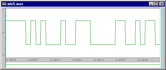
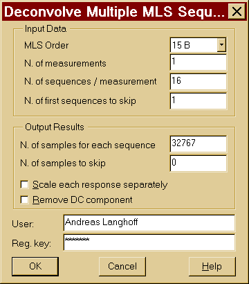
18	MLS method X(t) is a periodic binary signal obtained with a suitable shift-register, configured for maximum lenght of the period.
19	MLS deconvolution The re-recorded signal y(i) is cross-correlated with the excitation signal thanks to a fast Hadamard transform. The result is the required impulse response h(i), if the system was linear and time-invariant
20	MLS example
21	Example of a MLS impulse response
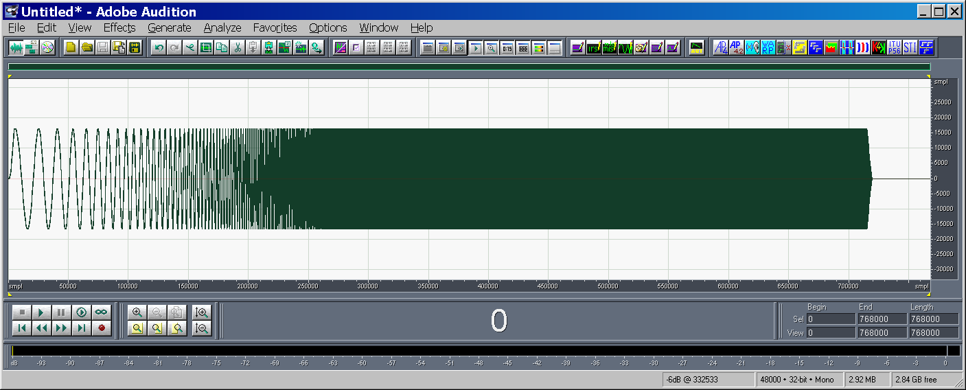
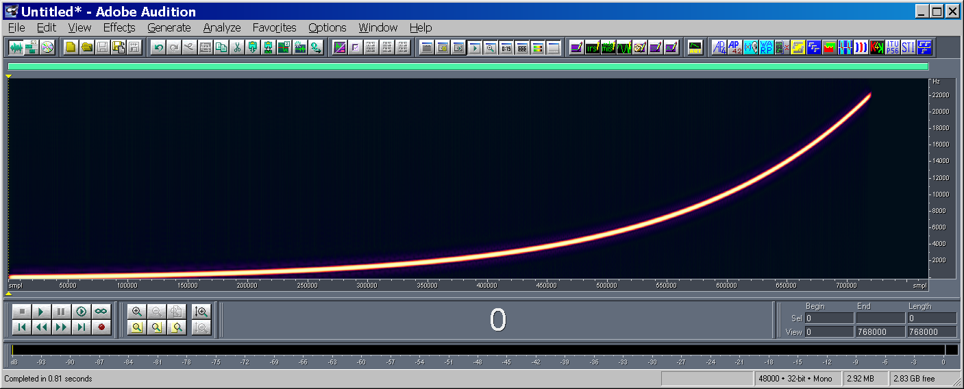
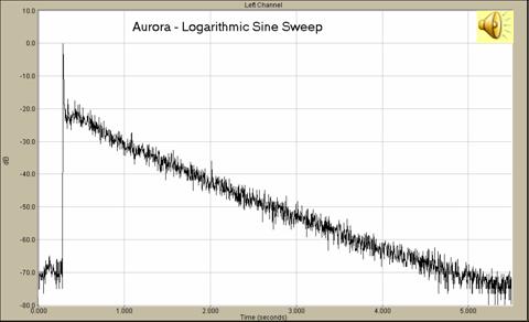
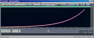
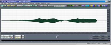
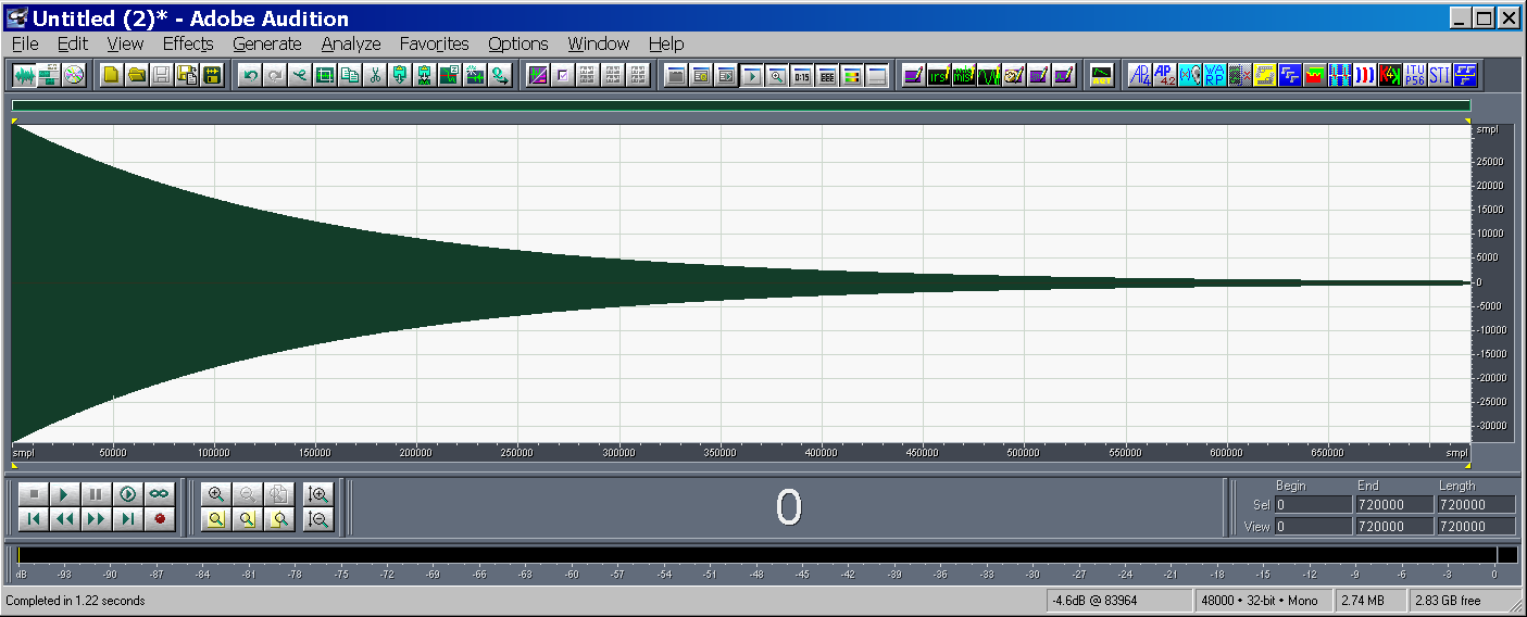
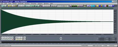
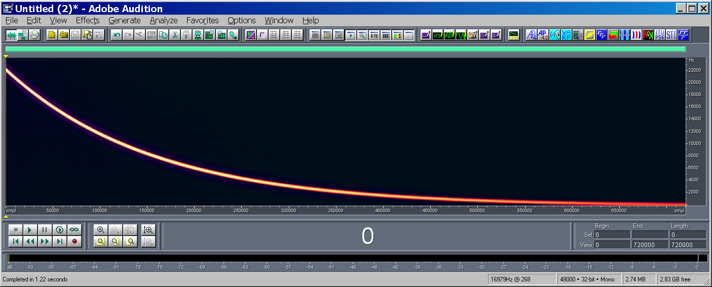
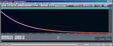
22	Exponential Sine Sweep method x(t) is a band-limited sinusoidal sweep signal, which frequency is varied exponentially with time, starting at f₁ and ending at f₂.
23	Test Signal – x(t)
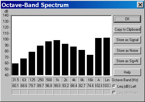
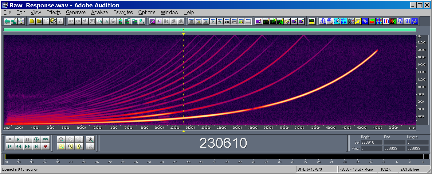
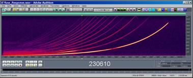
24	Measured signal - y(t) The not-linear behaviour of the loudspeaker causes many harmonics to appear
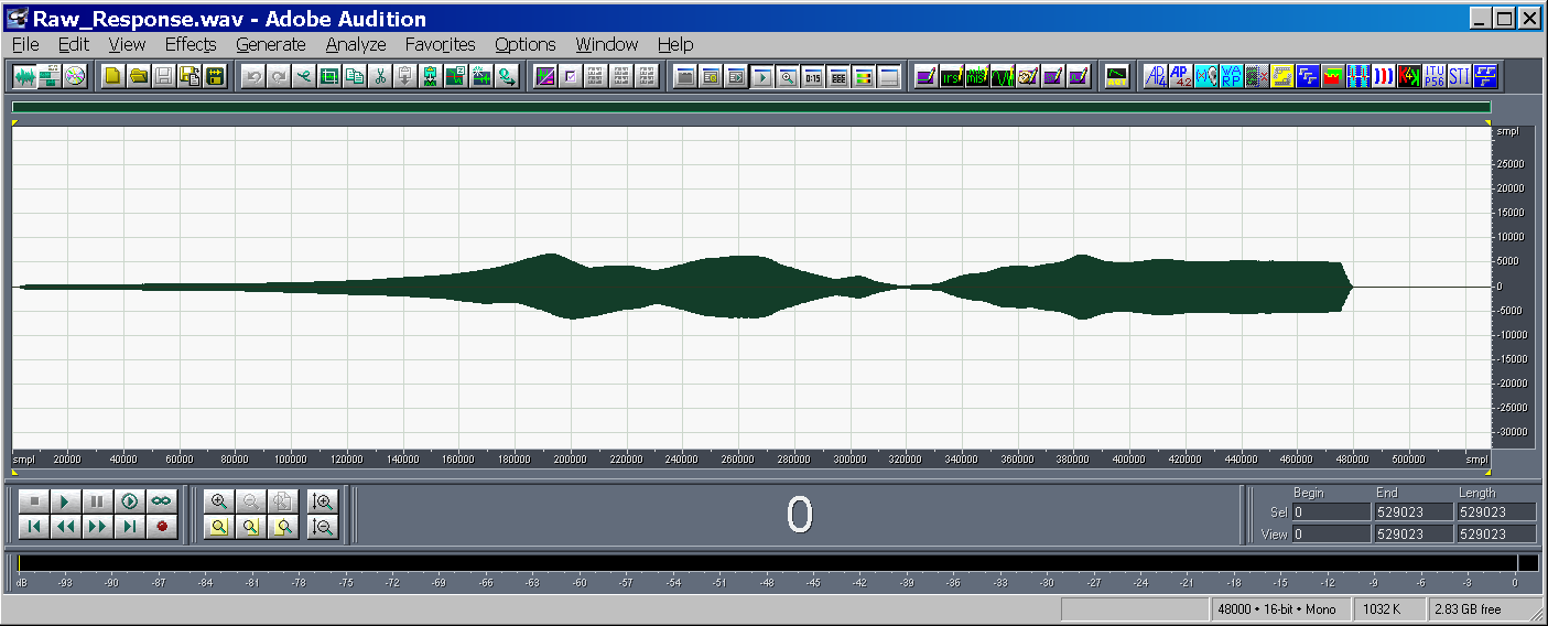
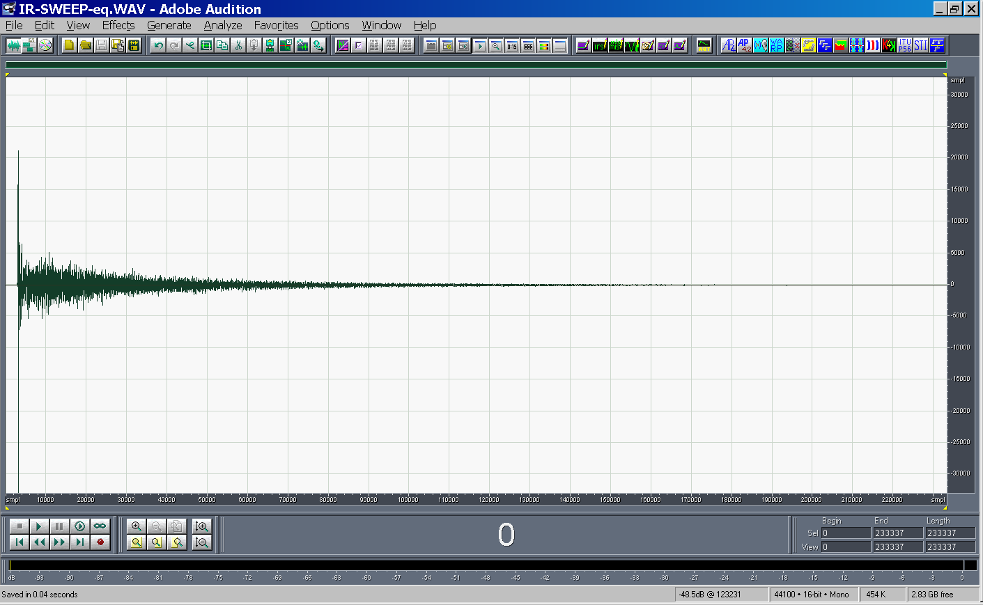
25	Inverse Filter – z(t) The deconvolution of the IR is obtained convolving the measured signal y(t) with the inverse filter z(t) [equalized, time-reversed x(t)]
26	Deconvolution of Exponential Sine Sweep The “time reversal mirror” technique is employed: the system’s impulse response is obtained by convolving the measured signal y(t) with the time-reversal of the test signal x(-t). As the log sine sweep does not have a “white” spectrum, proper equalization is required
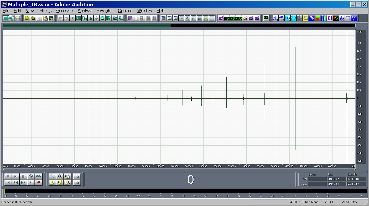
27	Result of the deconvolution The last impulse response is the linear one, the preceding are the harmonics distortion products of various orders
28	Maximum Length Sequence vs. Exp. Sine Sweep
29	Example of an ESS impulse response
30	Spatial analysis by directive microphones The initial approach was to use directive microphones for gathering some information about the spatial properties of the sound field “as perceived by the listener” Two apparently different approaches emerged: binaural dummy heads and pressure-velocity microphones:
31	IACC “objective” spatial parameter It was attempted to “quantify” the “spatiality” of a room by means of “objective” parameters, based on 2-channels impulse responses measured with directive microphones The most famous “spatial” parameter is IACC (Inter Aural Cross Correlation), based on binaural IR measurements
32	LF “objective” spatial parameter Other “spatial” parameters are the Lateral Energy ratio LF This is defined from a 2-channels impulse response, the first channel is a standard omni microphone, the second channel is a “figure-of-eight” microphone:
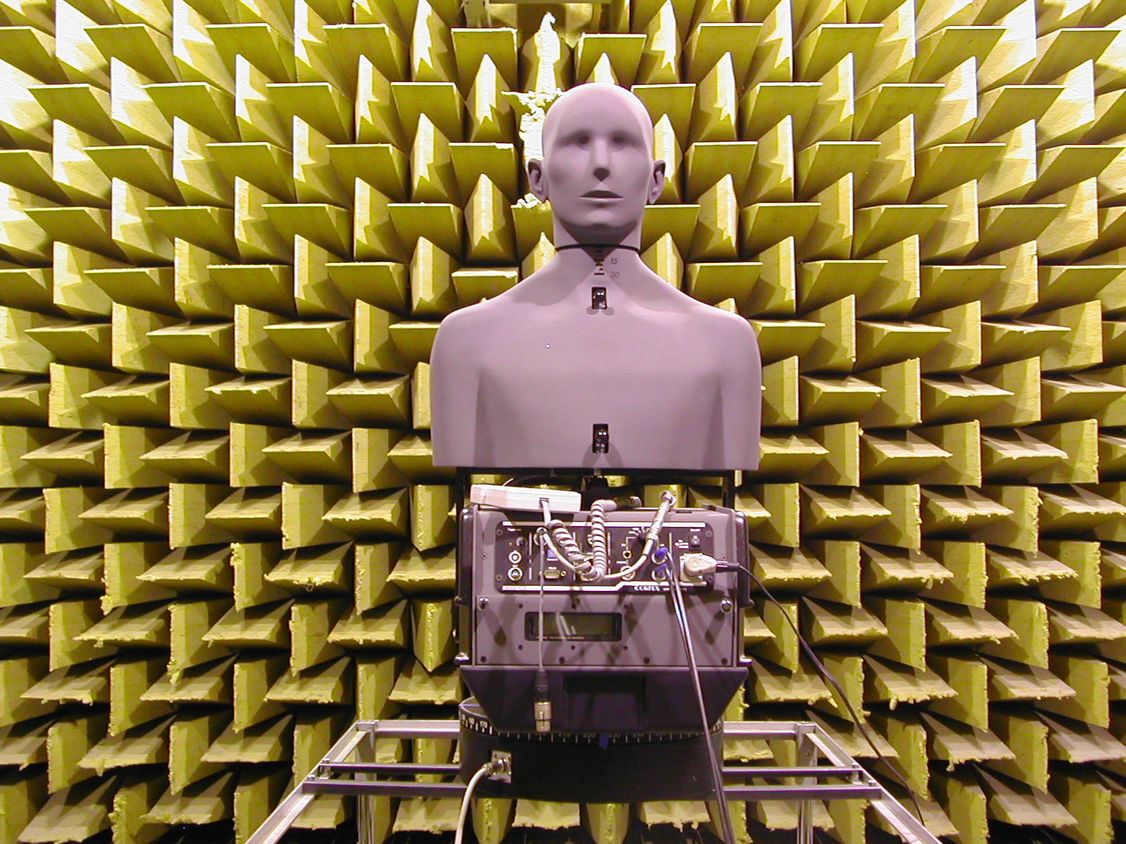
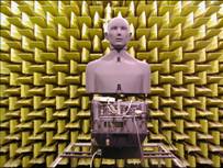
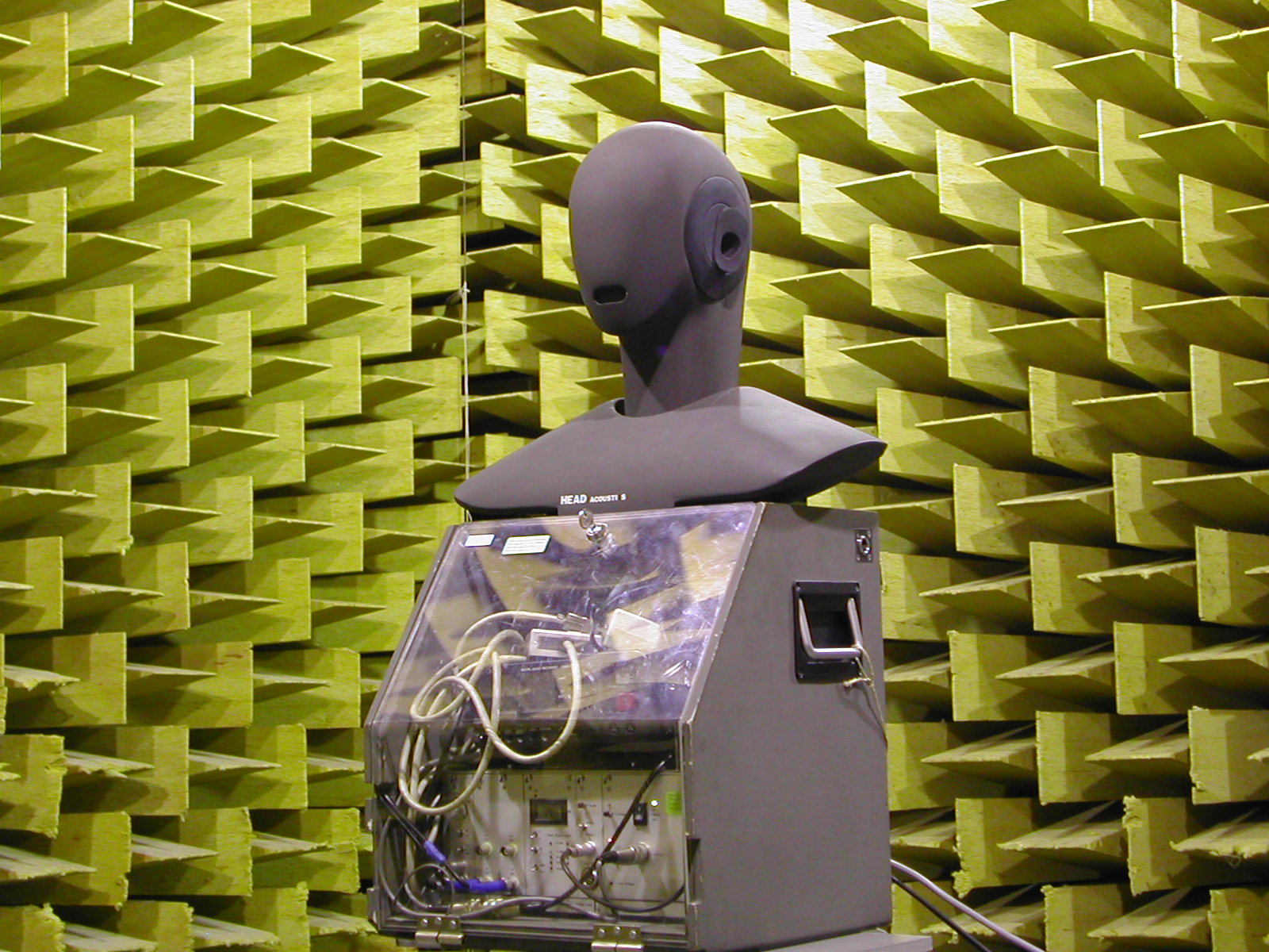
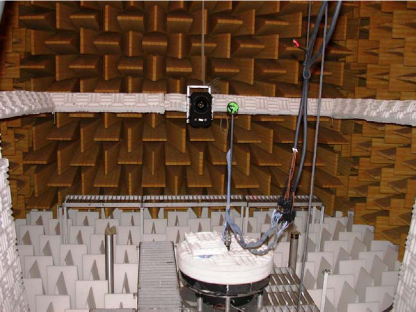
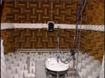
33	Are binaural measurents reproducible? Experiment performed in anechoic room - same loudspeaker, same source and receiver positions, 5 binaural dummy heads
34	Are binaural measurents reproducible? Diffuse field - huge difference among the 4 dummy heads
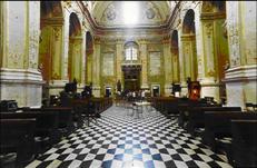
35	Are LF measurents reproducible? Experiment performed in the Auditorium of Parma - same loudspeaker, same source and receiver positions, 4 pressure-velocity microphones
36	Are LF measurents reproducible? At 25 m distance, the scatter is really big
37	3D Impulse Response (Gerzon, 1975)
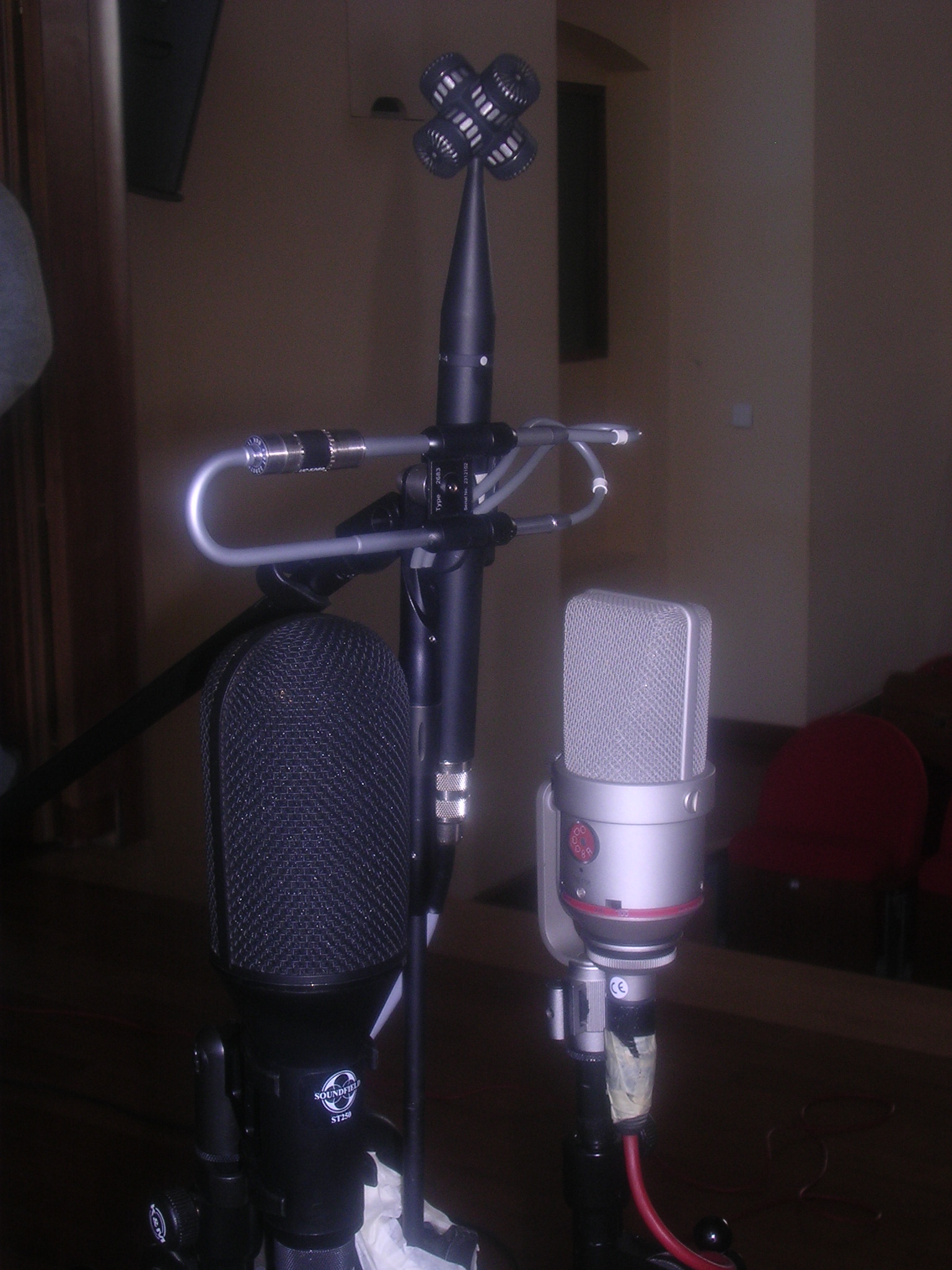
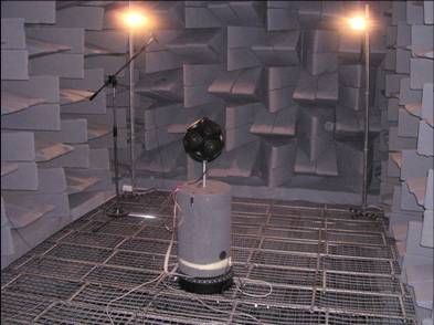
38	3D extension of the pressure-velocity measurements The Soundfield microphone allows for simultaneous measurements of the omnidirectional pressure and of the three cartesian components of particle velocity (figure-of-8 patterns)
39	The Waves project (2003) The original idea of Michael Gerzon was finally put in practice in 2003, thanks to the Israeli-based company WAVES More than 50 theatres all around the world were measured, capturing 3D IRs (4-channels B-format with a Soundfield microphone) The measurments did also include binaural impulse responses, and a circular-array of microphone positions More details on WWW.ACOUSTICS.NET
40	The Future
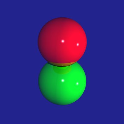
41	The Future Microphone arrays capable of synthesizing aribitrary directivity patterns Advanced spatial analysis of the sound field employing spherical harmonics (Ambisonics - 1° order or higher) Loudspeaker arrays capable of synthesizing arbitrary directivity patterns Generalized solution in which both the directivities of the source and of the receiver are represented as a spherical harmonics expansion
42	Directivity of transducers
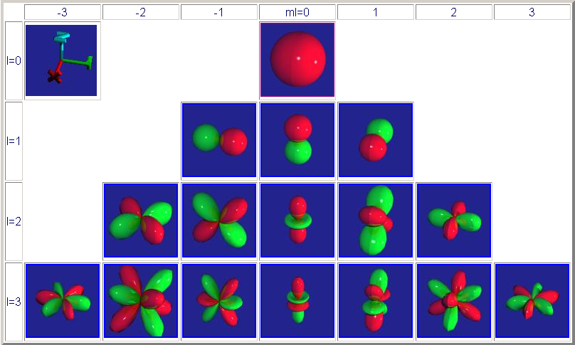
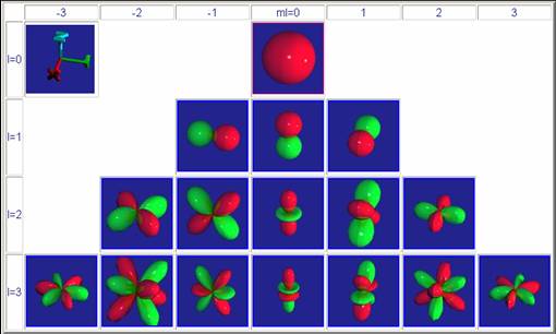
43	How to get better spatial resolution? The answer is simple: analyze the spatial distribution of both source and receiver by means of higher-order spherical harmonics expansion Spherical harmonics analysis is the equivalent, in space domain, of the Fourier analysis in time domain As a complex time-domain waveform can be though as the sum of a number of sinusoidal and cosinusoidal functions, so a complex spatial distribution around a given notional point can be expressed as the sum of a number of spherical harmonic functions
44	Higher-order spherical harmonics expansion
45	3°-order microphone (Trinnov - France) Arnoud Laborie developed a 24-capsule compact microphone array - by means of advanced digital filtering, spherical ahrmonic signals up to 3° order are obtained (16 channels)
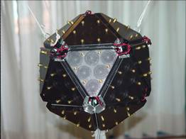
46	4°-order microphone (France Telecom) Jerome Daniel and Sebastien Moreau built samples of 32-capsules spherical arrays - these allow for extractions of microphone signals up to 4° order (25 channels)
47	Verification of high-order patterns Sebastien Moreau and Olivier Warusfel verified the directivity patterns of the 4°-order microphone array in the anechoic room of IRCAM (Paris)
48	What about source directivity ? Current 3D IR sampling is still based on the usage of an “omnidirectional” source The knowledge of the 3D IR measured in this way provide no information about the soundfield generated inside the room from a directive source (i.e., a musical instrument, a singer, etc.) Dave Malham suggested to represent also the source directivity with a set of spherical harmonics, called O-format - this is perfectly reciprocal to the representation of the microphone directivity with the B-format signals (Soundfield microphone). Consequently, a complete and reciprocal spatial transfer function can be defined, employing a 4-channels O-format source and a 4-channels B-format receiver:
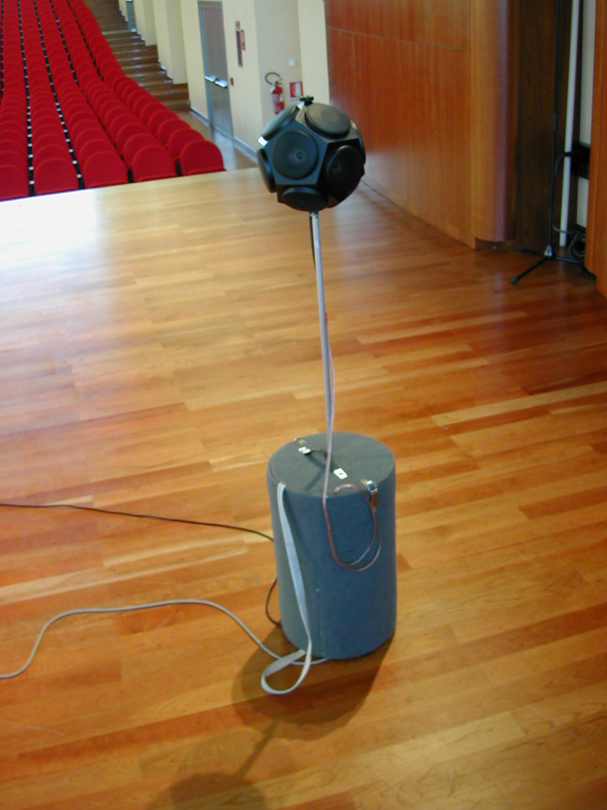
49	Directivity of transducers LookLine D200 dodechaedron
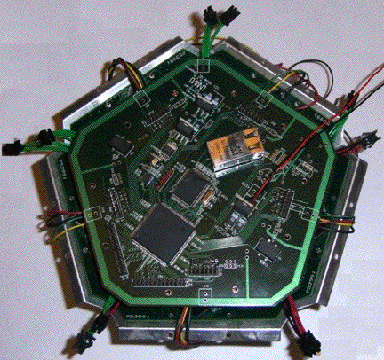
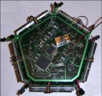
50	High-order sound source Adrian Freed, Peter Kassakian, and David Wessel (CNMAT) developed a new 120-loudspeakers, digitally controlled sound source, capable of synthesizing sound emission according to spherical harmonics patterns up to 5° order.
51	Technical details of high-order source Class-D embedded amplifiers
52	Accuracy of spatial synthesis The spatial reconstruction error of a 120-loudspeakers array is frequency dependant, as shown here:
53	Complete high-order MIMO method Employing massive arrays of transducers, it will be feasible to sample the acoustical temporal-spatial transfer function of a room Currently available hardware and software tools make this practical only up to 4° order, which means 25 inputs and 25 outputs A complete measurement for a given source-receiver position pair takes approximately 10 minutes (25 sine sweeps of 15s each are generated one after the other, while all the microphone signals are sampled simultaneously) However, it has been seen that real-world sources can be already approximated quite well with 2°-order functions, and even the human HRTF directivites are reasonally approximated with 3°-order functions.
54	Conclusions The sine sweep method revealed to be systematically superior to the MLS method for measuring electroacoustical impulse responses Traditional methods for measuring “spatial parameters” (IACC, LF) proved to be unreliable and do not provide complete information The 1°-order Ambisonics method can be used for generating and recording sound with a limited amount of spatial information For obtaining better spatial resolution, High-Order Ambisonics can be used, limiting the spherical-harmonics expansion to a reasonable order (2°, 3° or 4°). Experimental hardware and software tools have been developed (mainly in France, but also in USA), allowing to build an inexpensive complete measurement system