|
1
|
|
|
2
|
|
|
3
|
|
|
4
|
|
|
5
|
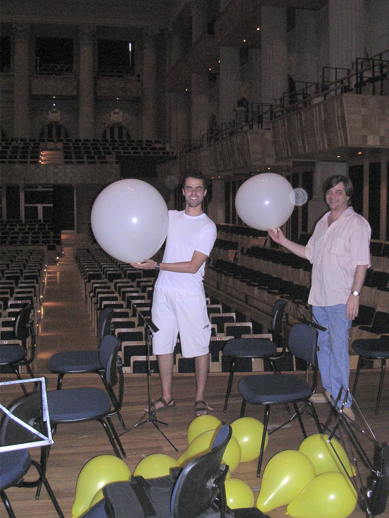
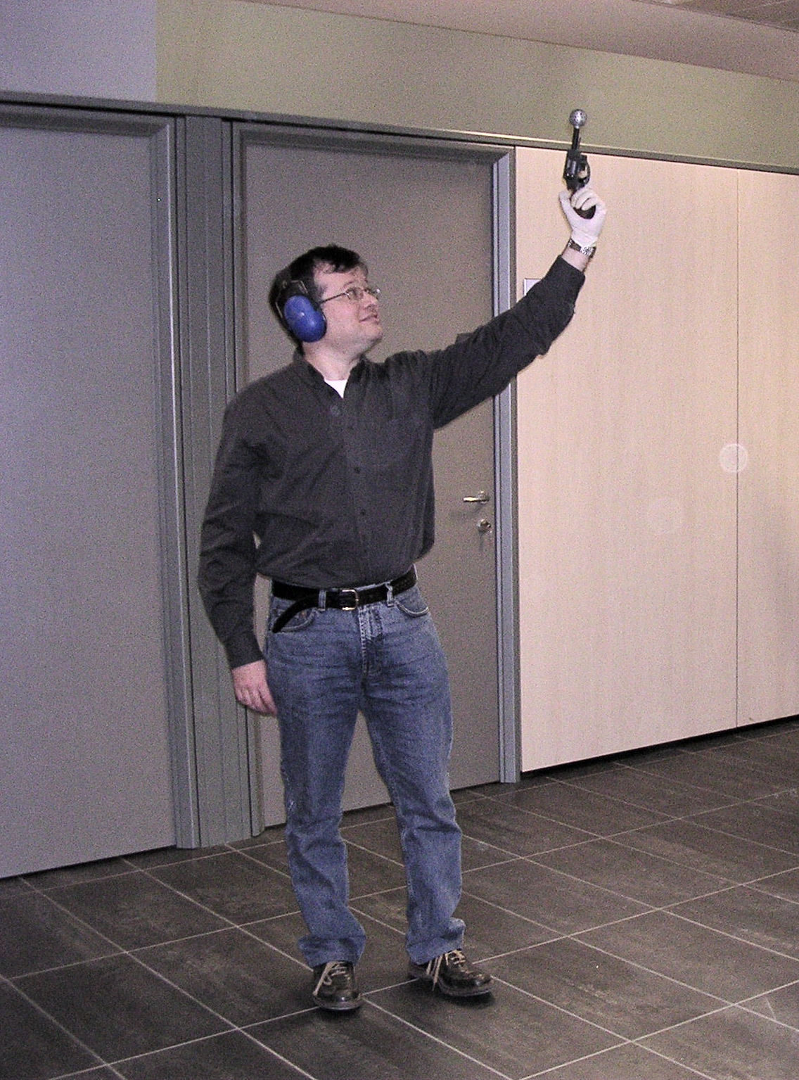
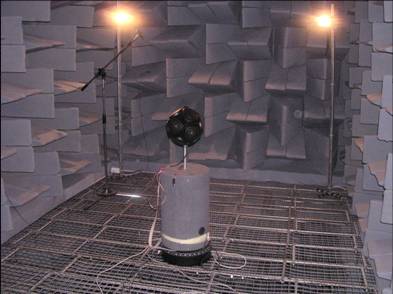
- Pulsive sources: ballons, blank pistol
|
|
6
|
|
|
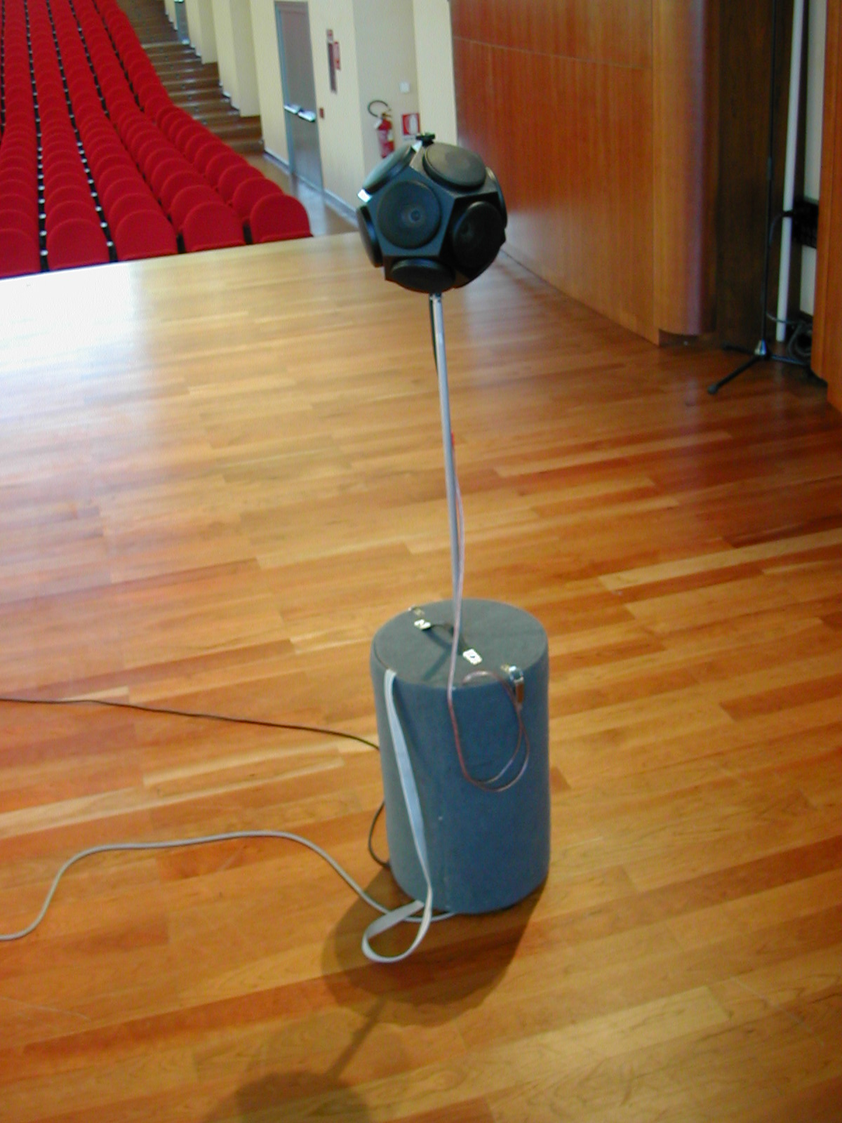
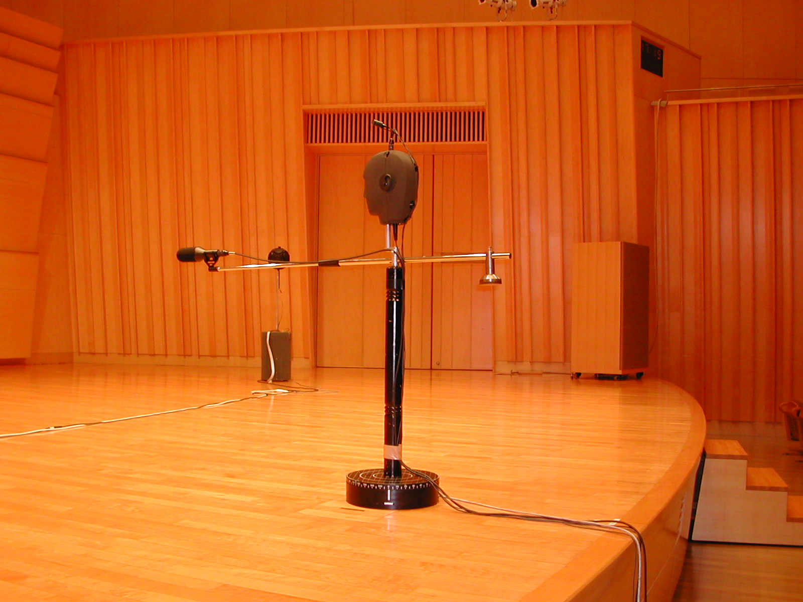
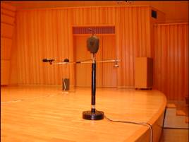
7
|
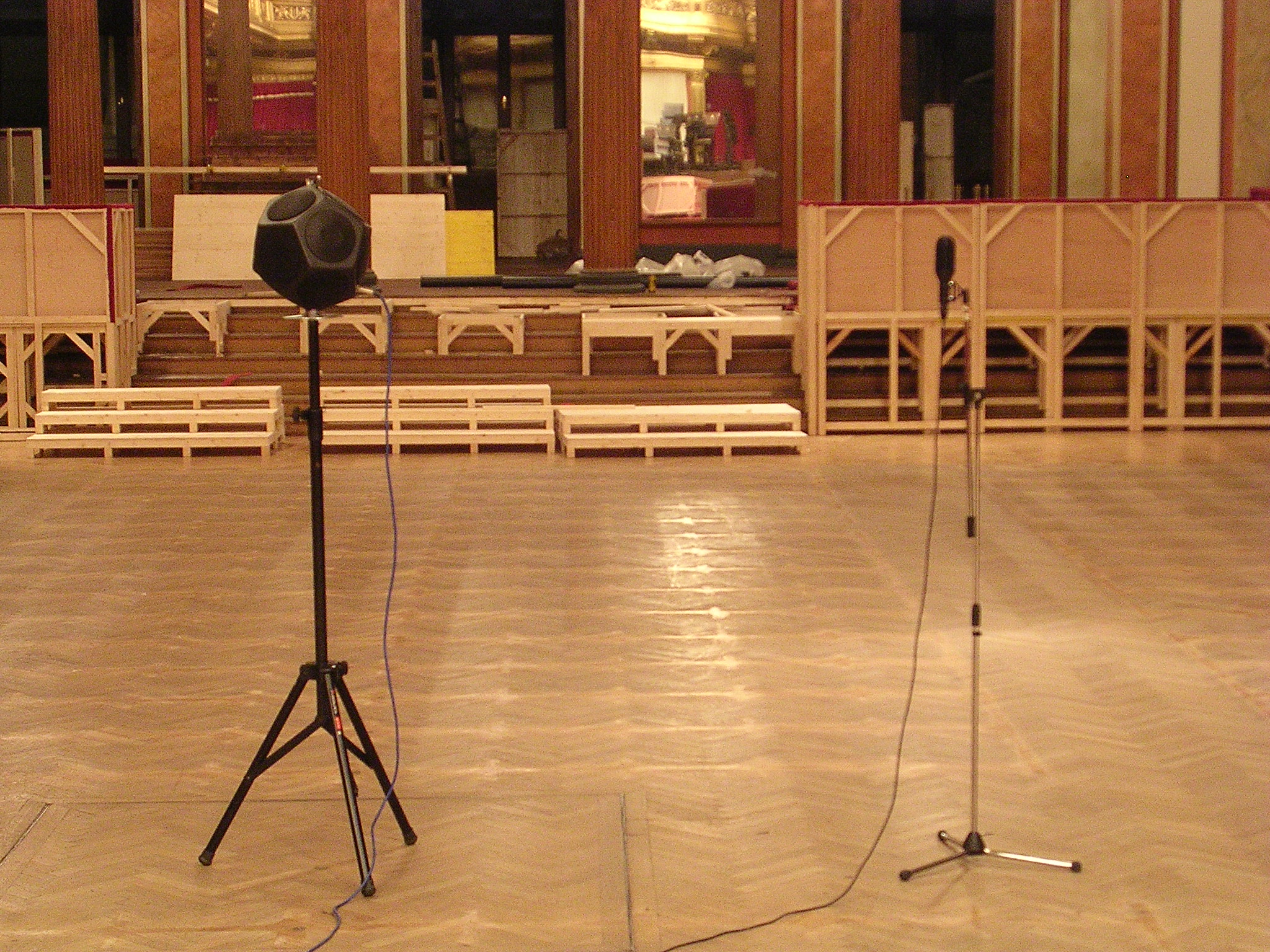
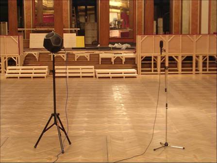
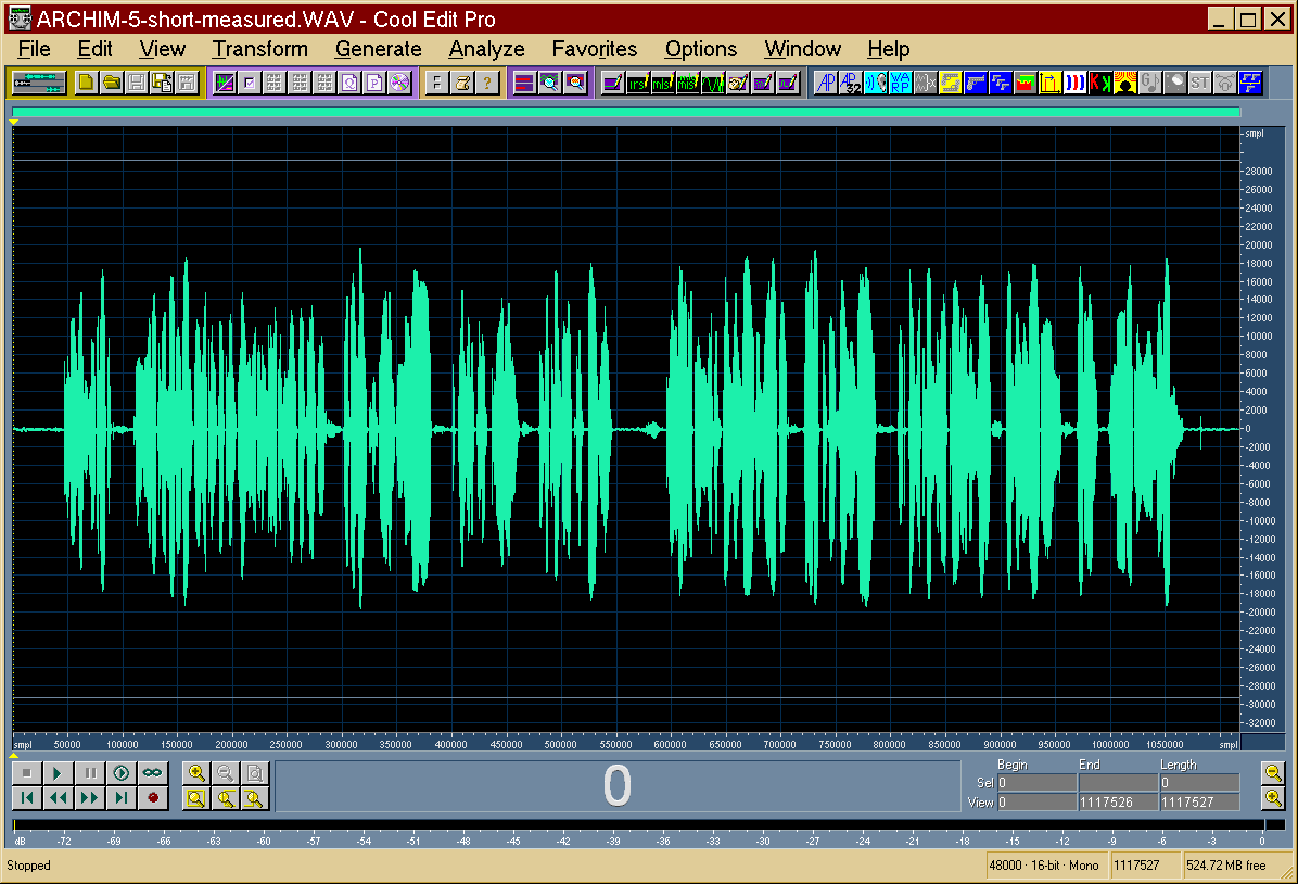
- A loudspeaker is fed with a special test signal x(t), while a microphone
records the room response
- A proper deconvolution technique is required for retrieving the impulse
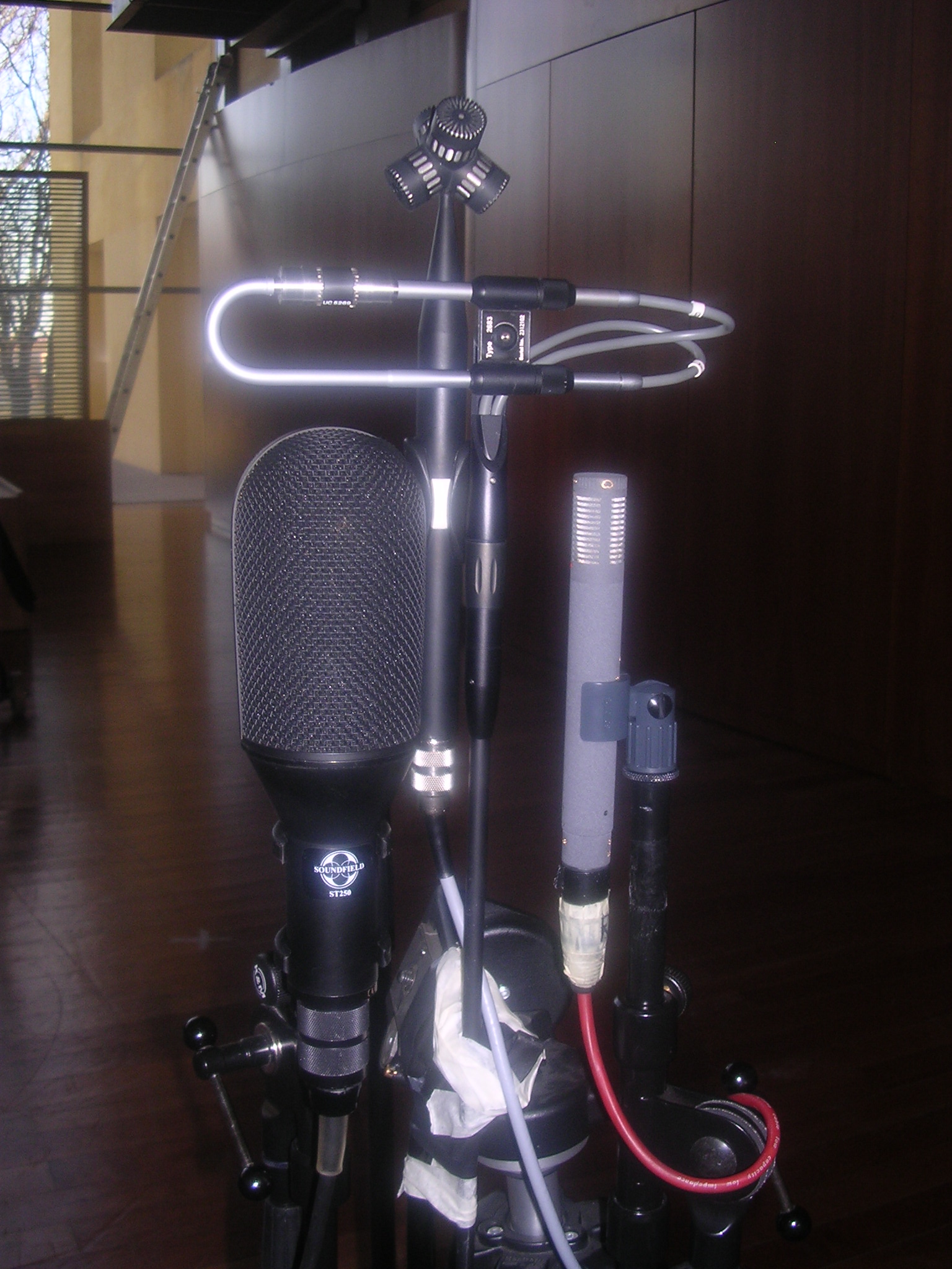
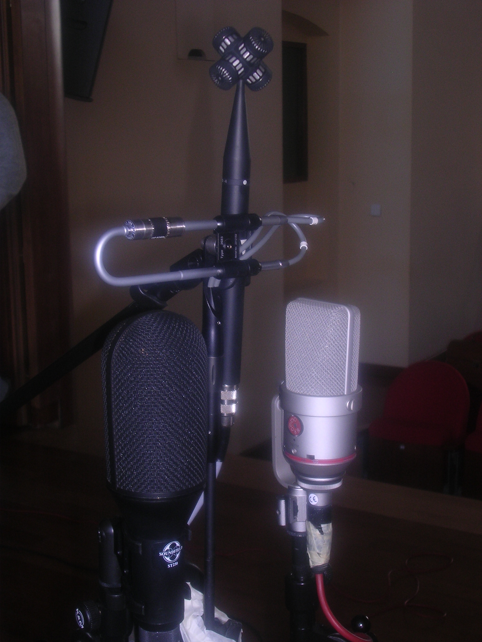
response h(t) from the recorded signal y(t)
|
|
8
|
- The desidered result is the linear impulse response of the acoustic
propagation h(t). It can be recovered by knowing the test signal x(t)
and the measured system output y(t).
- It is necessary to exclude the effect of the not-linear part K and of
the background noise n(t).
|
|
9
|
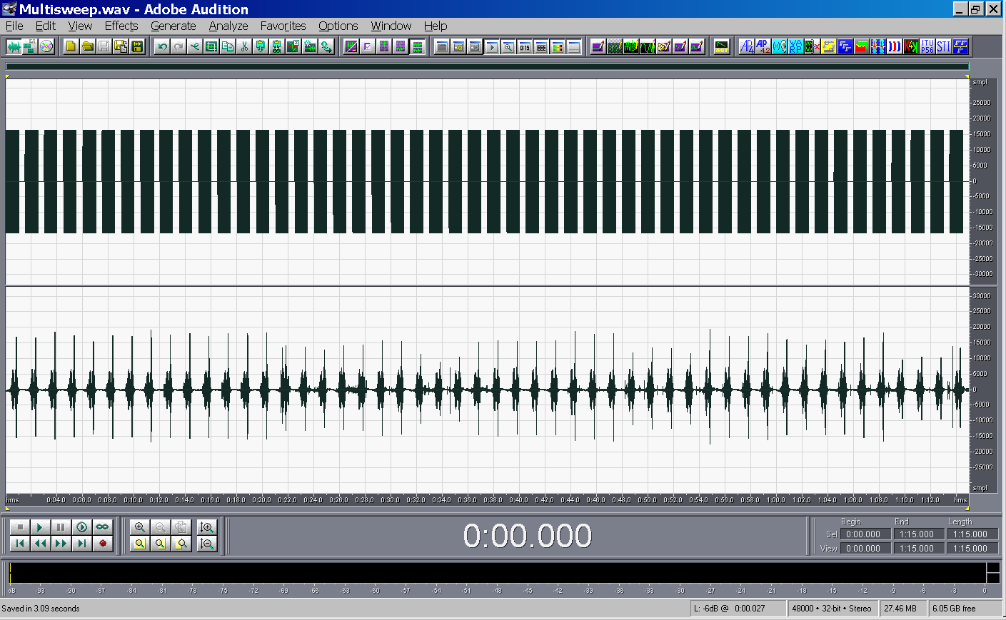
- Different types of test signals have been developed, providing good
immunity to background noise and easy deconvolution of the impulse
response:
- MLS (Maximum Lenght Sequence, pseudo-random white noise)
- TDS (Time Delay Spectrometry, which basically is simply a linear sine
sweep, also known in Japan as “stretched pulse” and in Europe as
“chirp”)
- ESS (Exponential Sine Sweep)
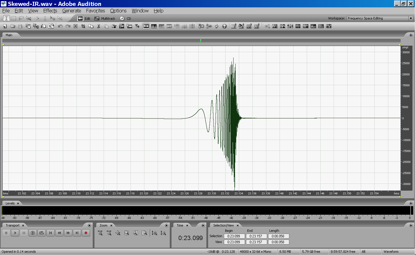
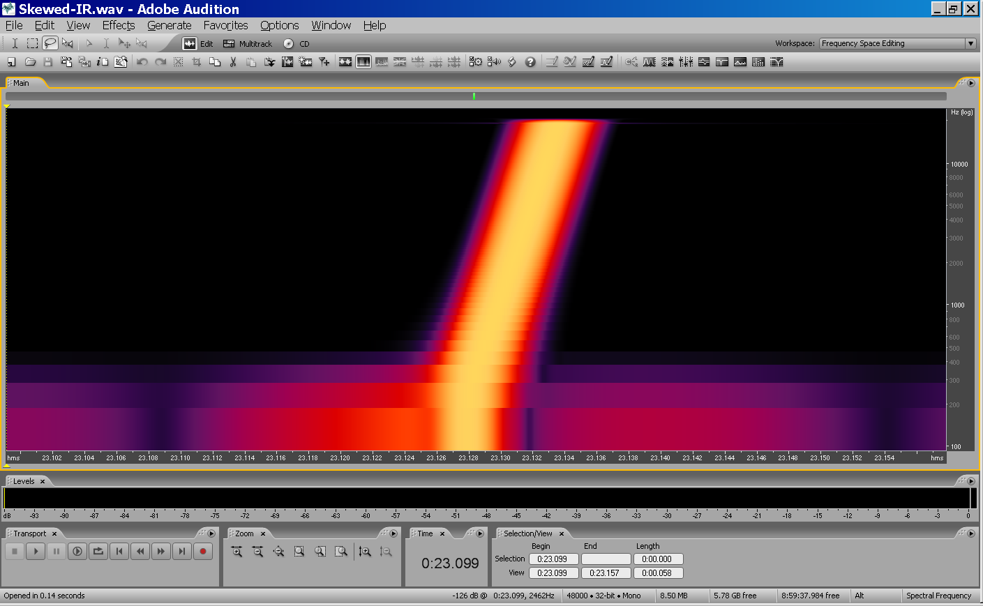
- Each of these test signals can be employed with different deconvolution
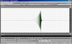
techniques, resulting in a number of “different” measurement methods
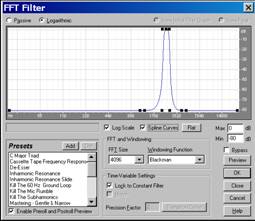
- Due to theoretical and practical considerations, the preference is
nowadays generally oriented for the usage of ESS with not-circular
deconvolution
|
|
10
|
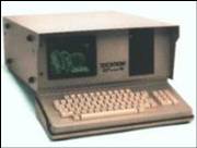
- MLSSA was the first apparatus for measuring impulse responses with MLS
|
|
11
|
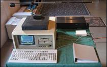
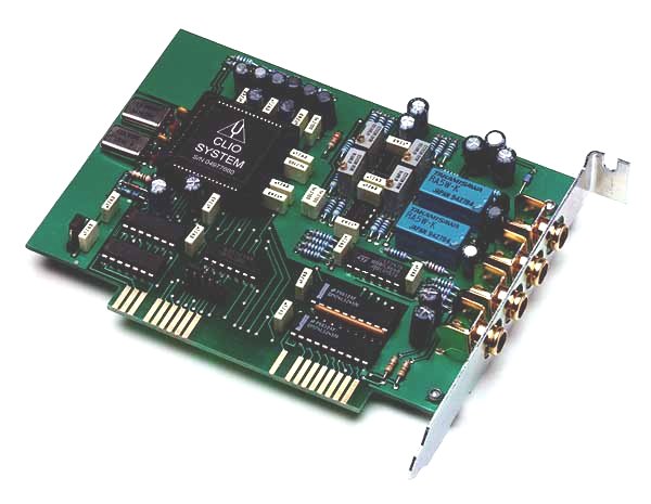
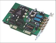
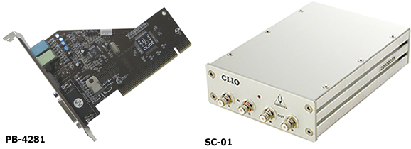
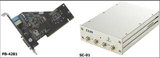
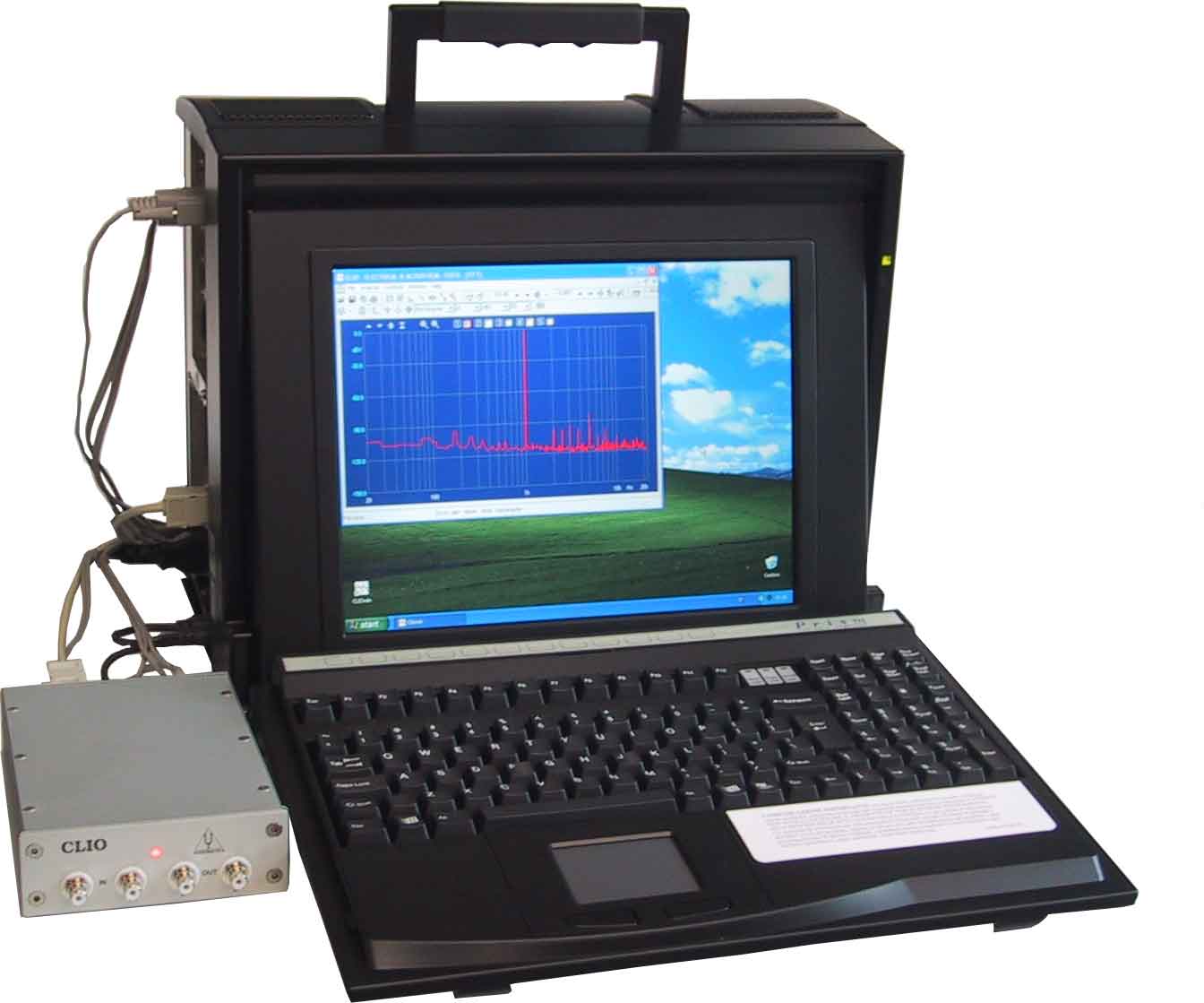
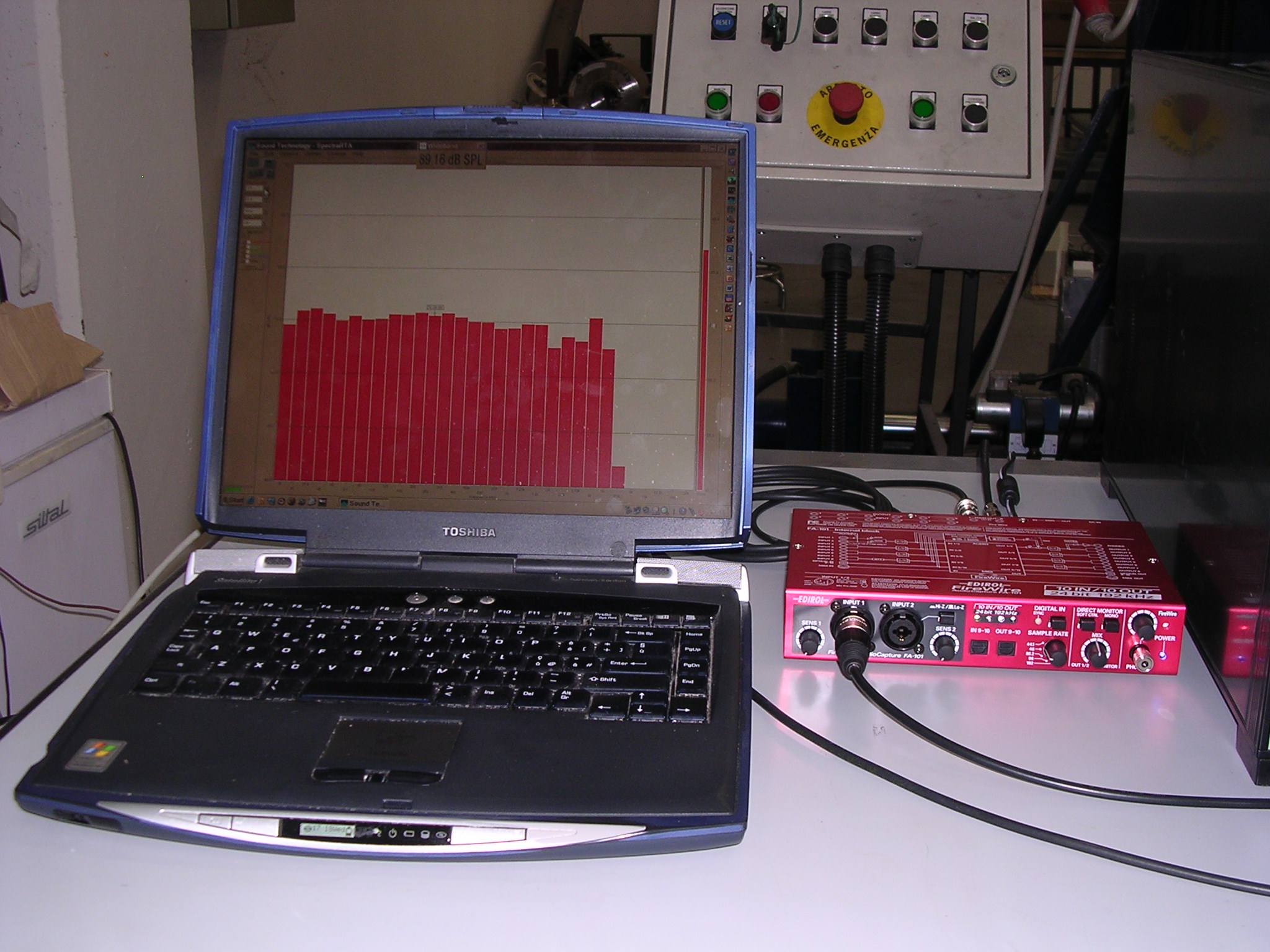
- The Italian-made CLIO system has superseded MLSSA for most low-cost
electroacoustics applications (measurement of loudspeakers, quality
control)
|
|
12
|
- Techron TEF 10 was the first apparatus for measuring impulse responses
with TDS
- Subsequent versions (TEF 20, TEF 25) also support MLS
|
|
13
|
|
|
14
|
|
|
15
|
|
|
16
|
|
|
17
|
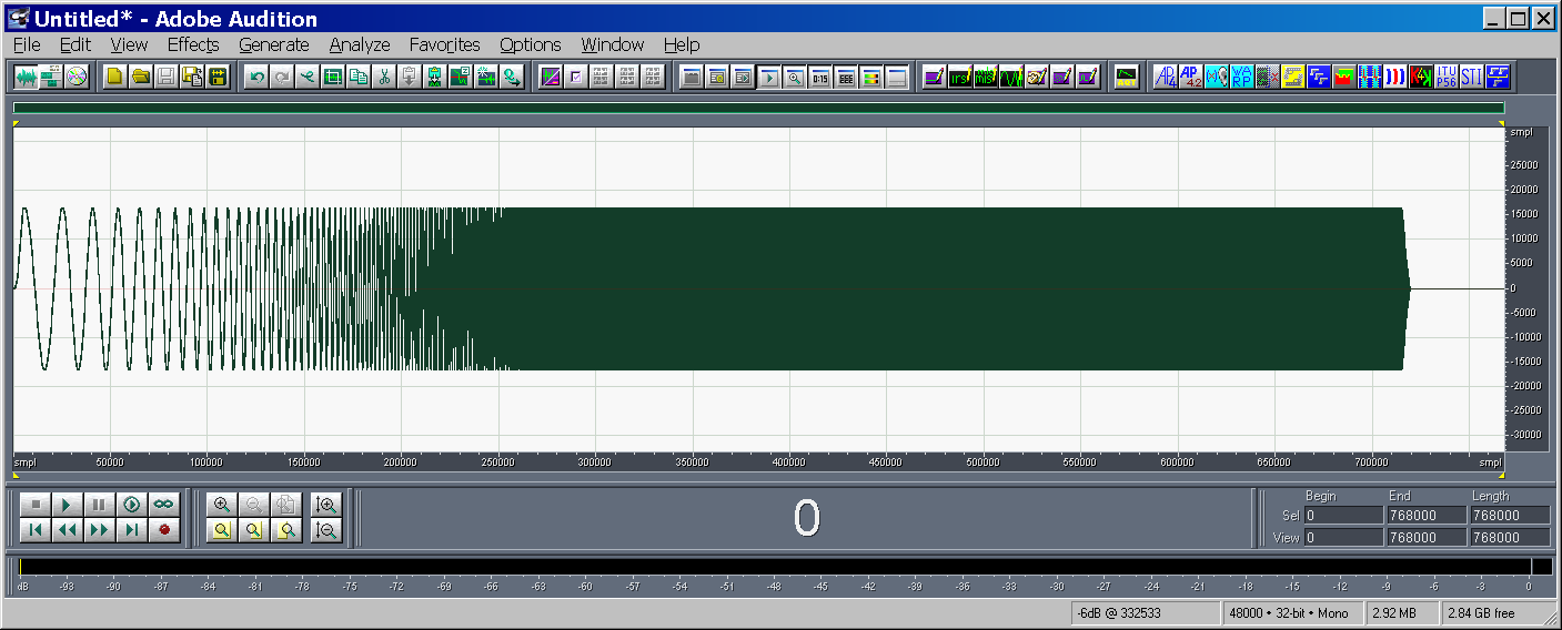
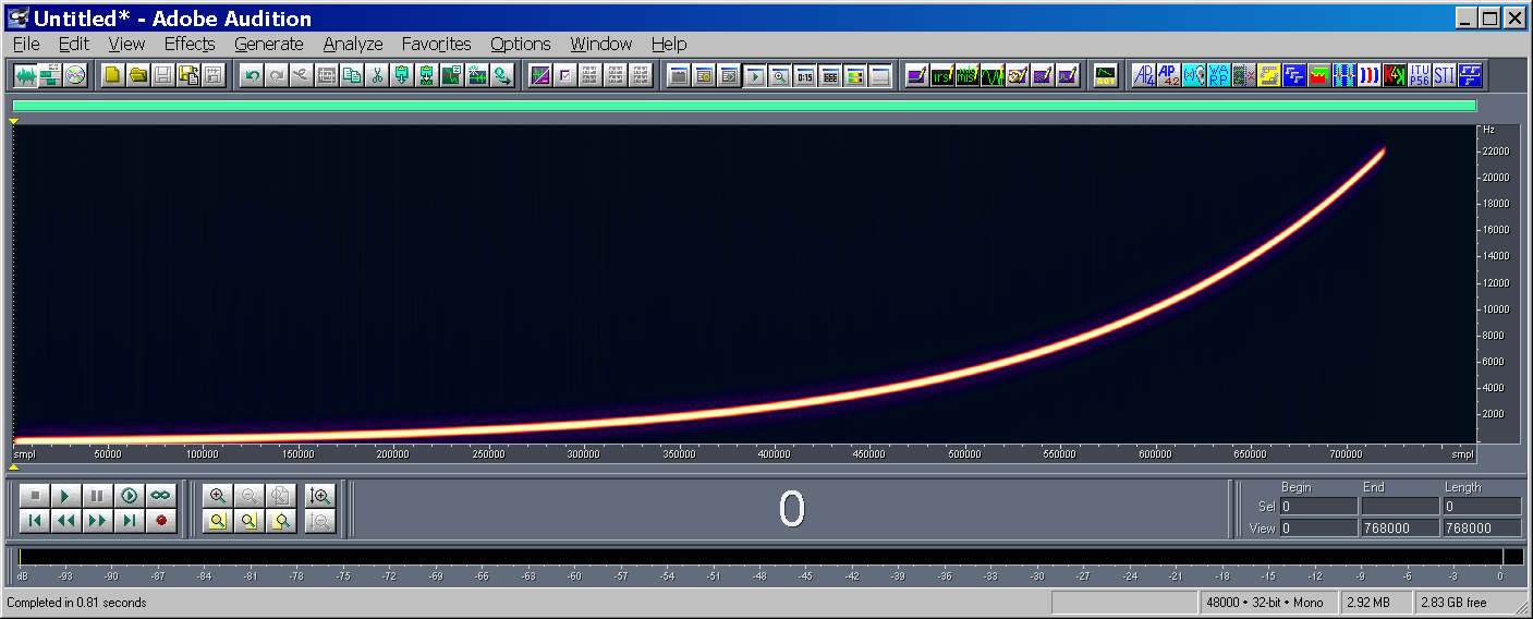
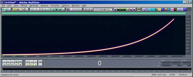
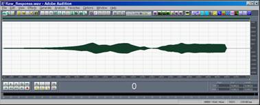
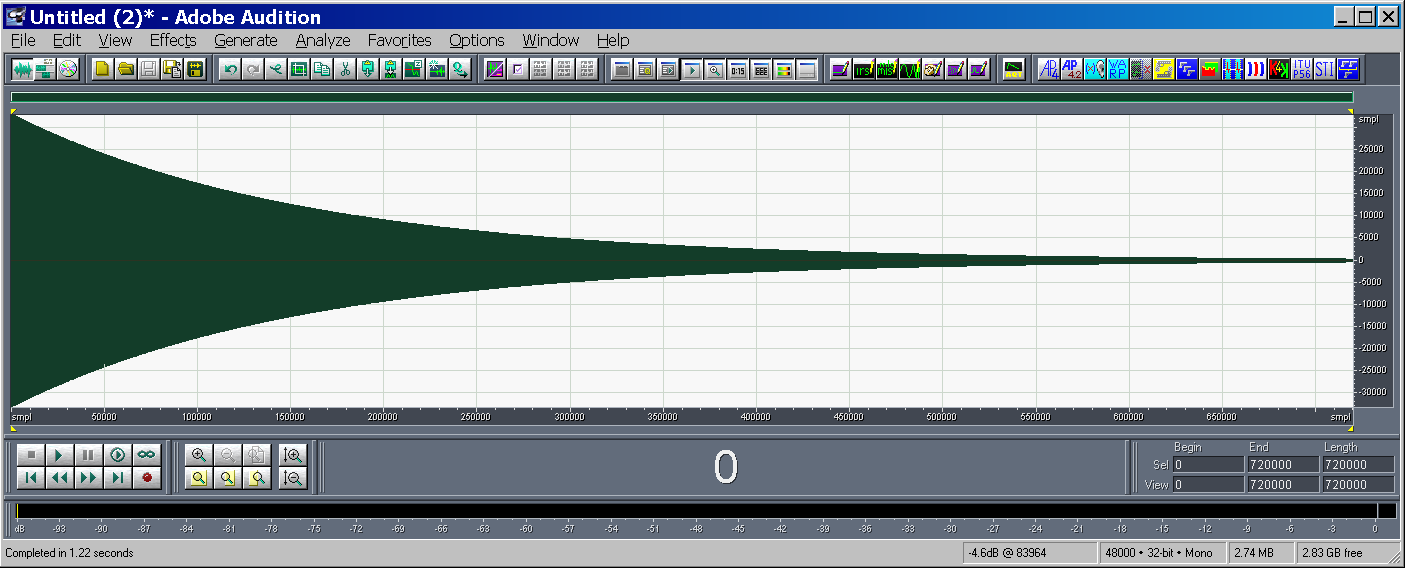
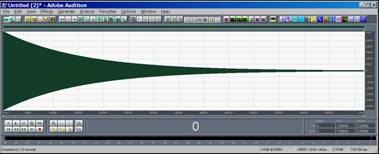
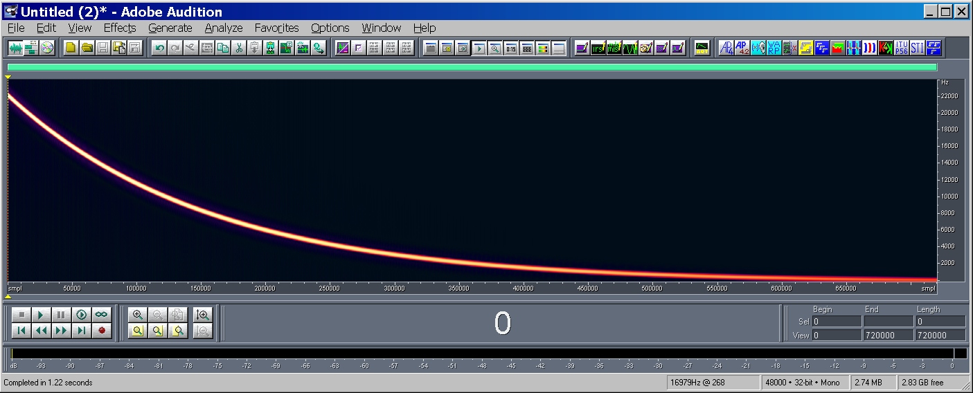
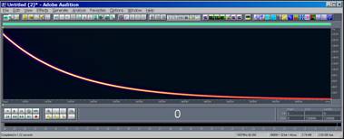
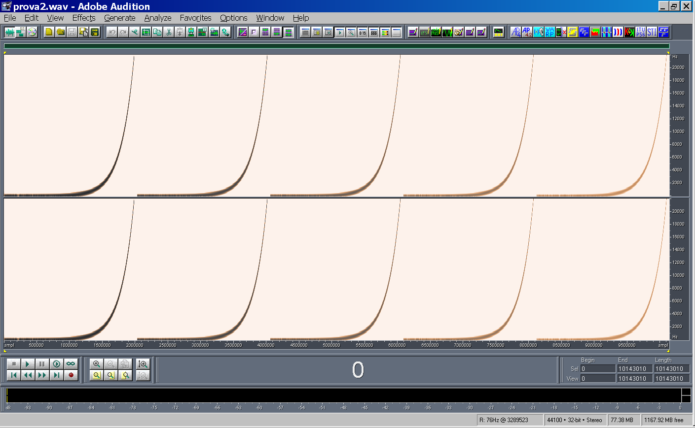
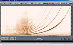
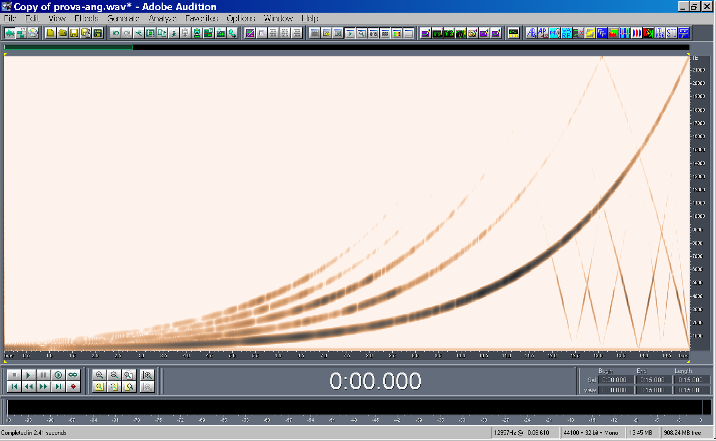
- x(t) is a band-limited sinusoidal
sweep signal, which frequency is varied exponentially with time,
starting at f1 and ending at f2.
|
|
18
|
|
|
19
|
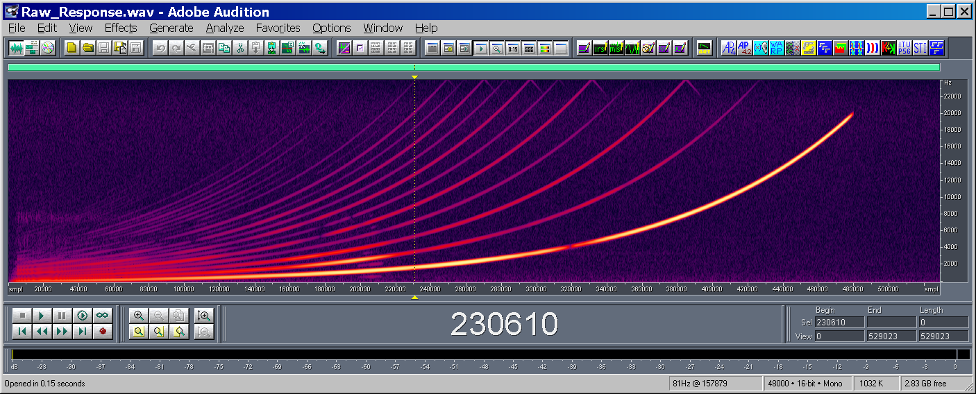
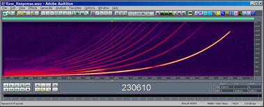
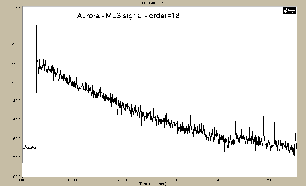
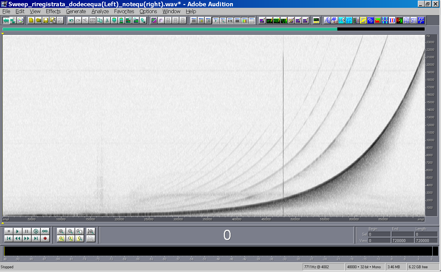
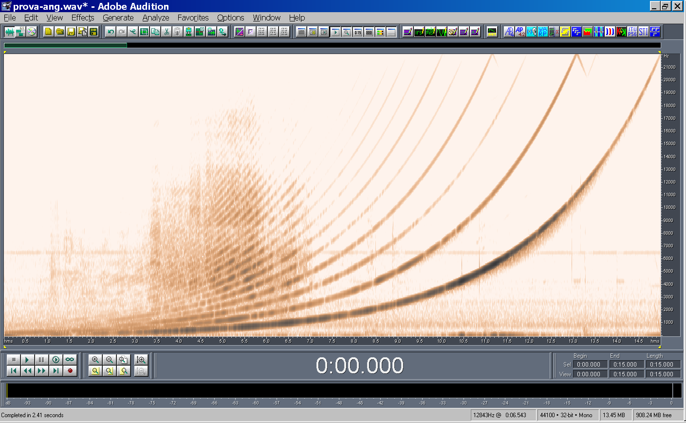
- The not-linear behaviour of the loudspeaker causes many harmonics to
appear
|
|
20
|
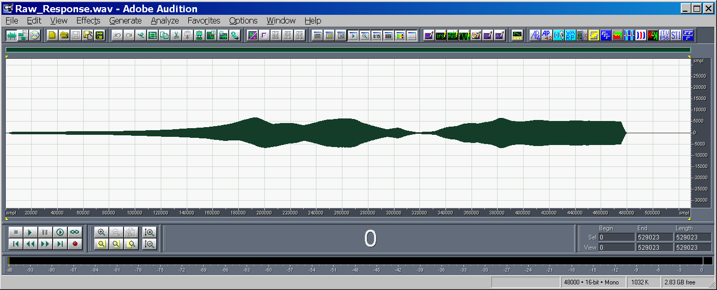
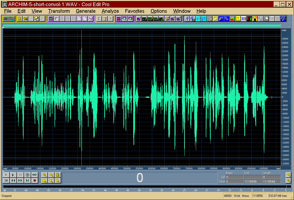
- The deconvolution of the IR is obtained convolving the measured signal
y(t) with the inverse filter z(t) [equalized, time-reversed x(t)]
|
|
21
|
- The “time reversal mirror” technique is employed: the system’s impulse
response is obtained by convolving the measured signal y(t) with the
time-reversal of the test signal x(-t). As the log sine sweep does not
have a “white” spectrum, proper equalization is required
|
|
22
|
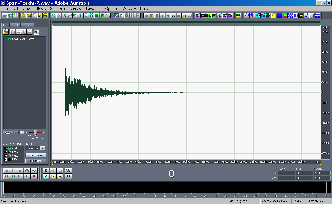
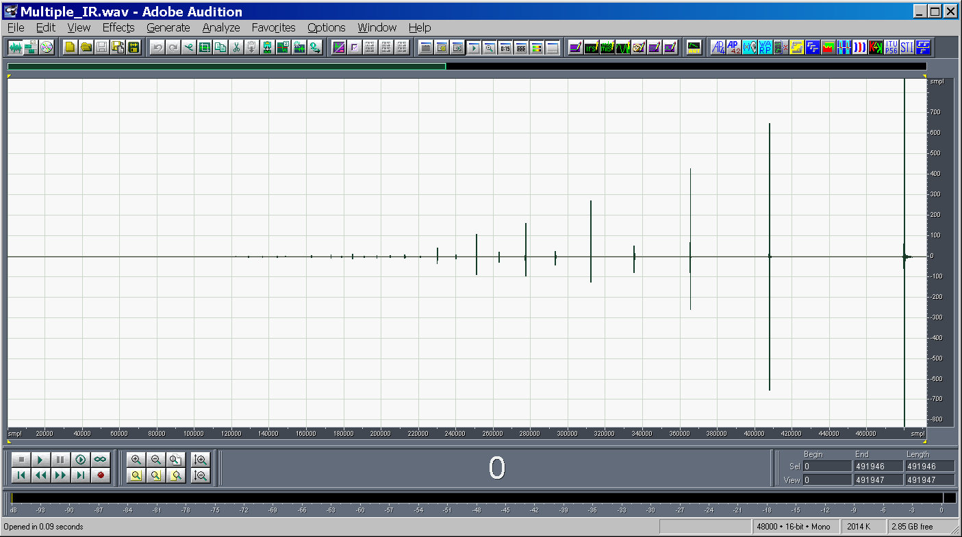
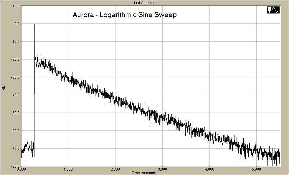
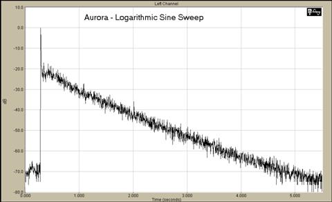
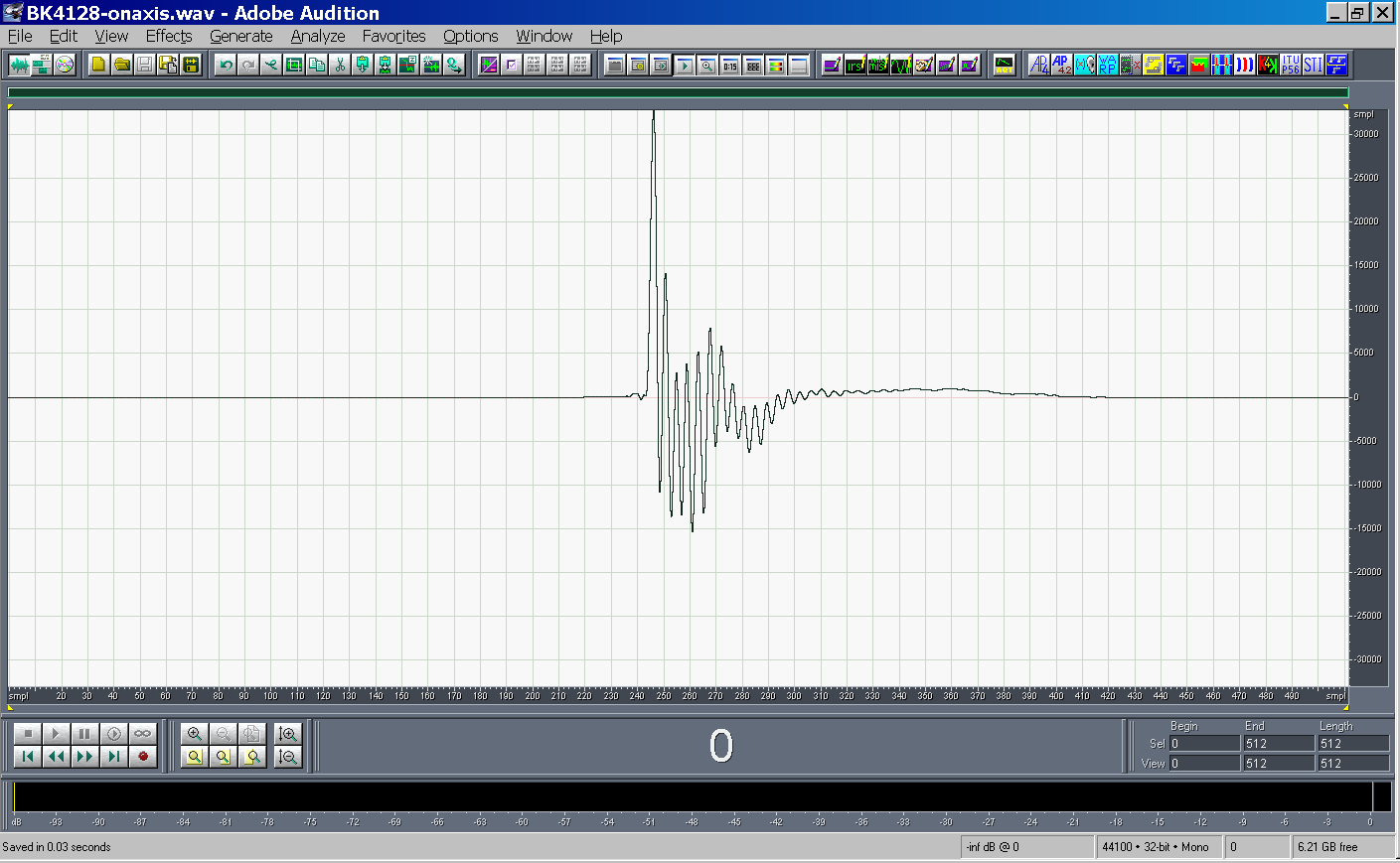
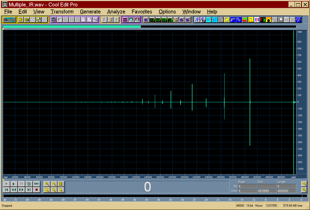
- The last impulse response is the linear one, the preceding are the
harmonics distortion products of various orders
|
|
23
|
|
|
24
|
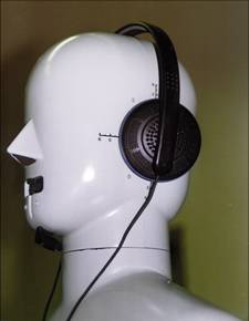
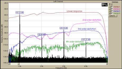
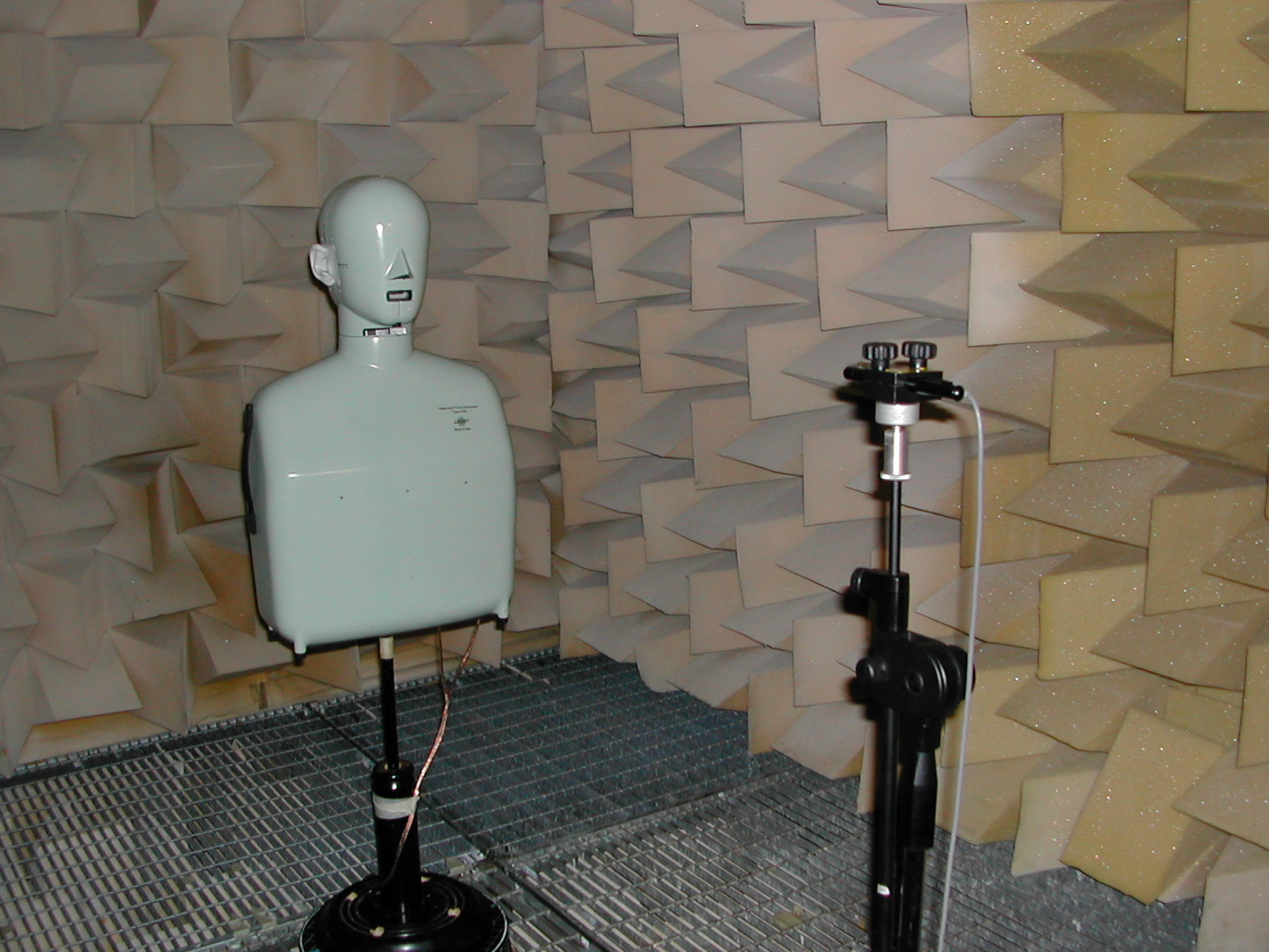
- A headphone was driven with a 1 V RMS signal, causing severe distortion
in the small loudspeaker.
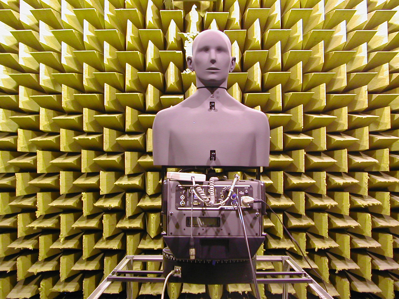
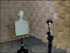
- The measurement was made placing the headphone on a dummy head.
- Measurements: ESS and traditional sine at 1 kHz
|
|
25
|
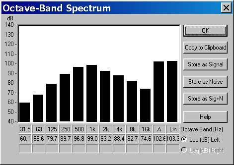
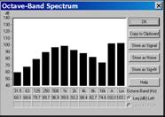
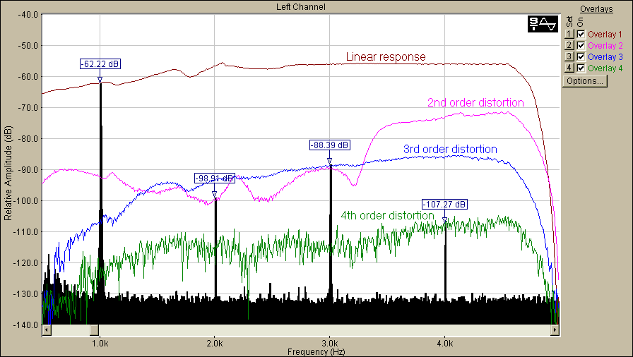
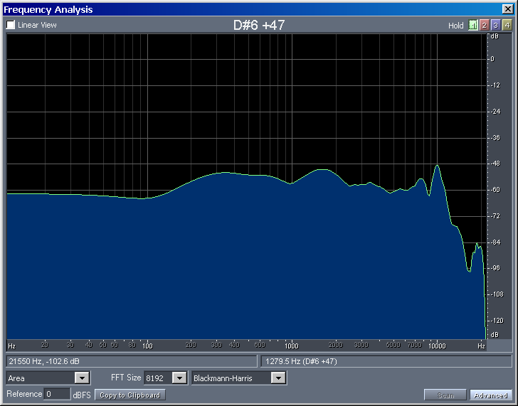
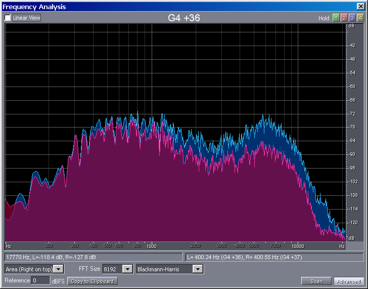
- Comparison between:
- traditional distortion
measurement with fixed-frequency sine (the black histogram)
- the new exponential sweep (the 4 narrow, coloured lines)
|
|
26
|
- The initial approach was to use directive microphones for gathering some
information about the spatial properties of the sound field “as
perceived by the listener”
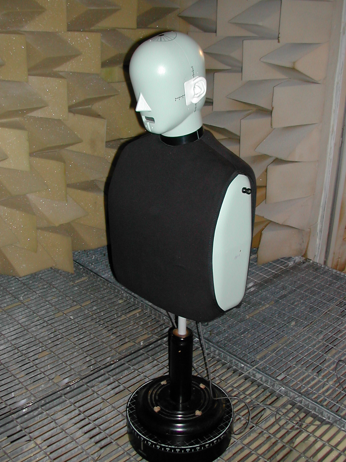
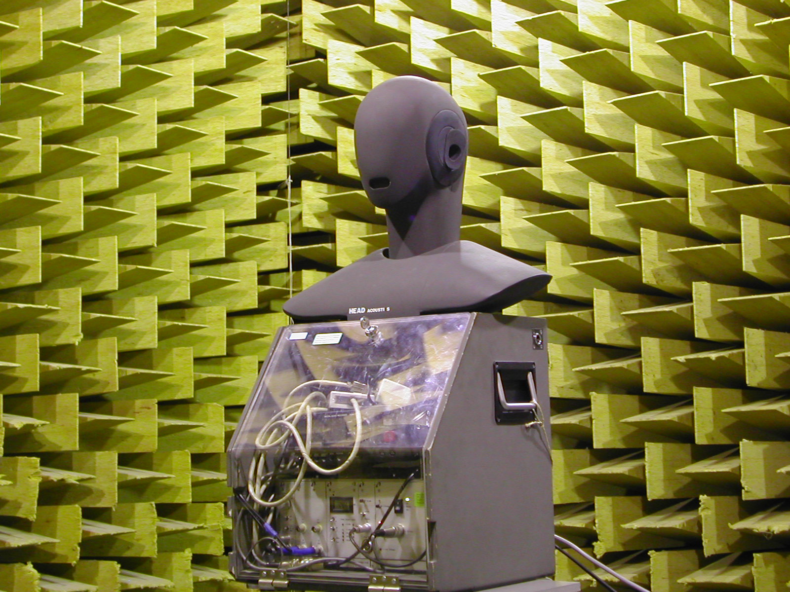
- Two apparently different approaches emerged: binaural dummy heads and
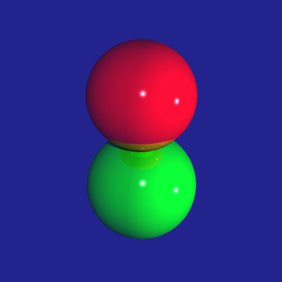
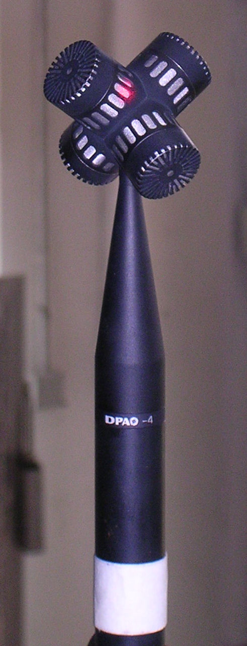
pressure-velocity microphones:
|
|
27
|
- It was attempted to “quantify” the “spatiality” of a room by means of
“objective” parameters, based on 2-channels impulse responses measured
with directive microphones
- The most famous “spatial” parameter is IACC (Inter Aural Cross
Correlation), based on binaural IR measurements
|
|
28
|
- Another “spatial” parameter is the Lateral Fraction LF
- This is defined from a 2-channels impulse response, the first channel is
a standard omni microphone, the second channel is a “figure-of-eight”
microphone:
|
|
29
|
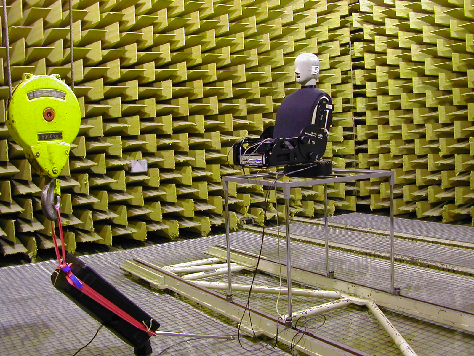
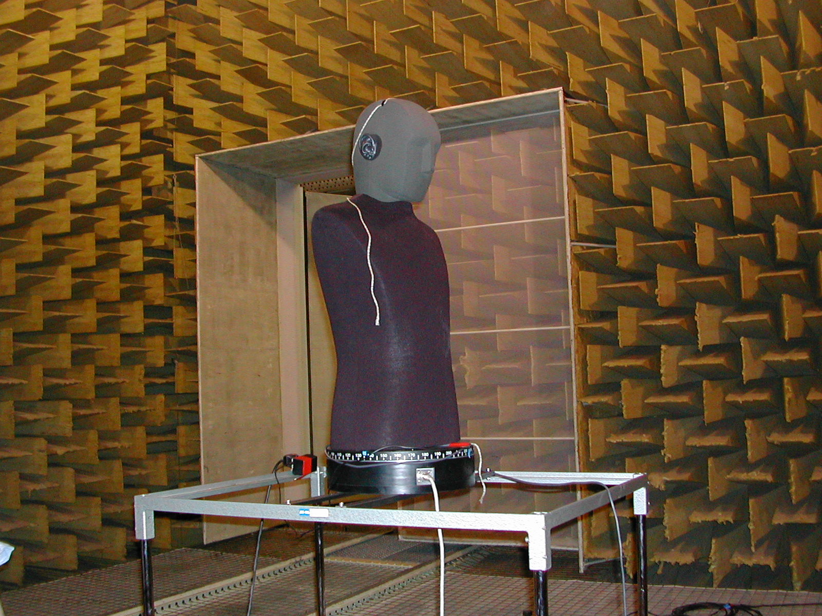
- Experiment performed in anechoic room - same loudspeaker, same source
and receiver positions, 5 binaural dummy heads
|
|
30
|
- Diffuse field - huge difference among the 4 dummy heads
|
|
31
|
- Experiment performed in the Auditorium of Parma - same loudspeaker, same
source and receiver positions, 4 pressure-velocity microphones
|
|
32
|
- At 25 m distance, the scatter is really big
|
|
33
|
|
|
34
|
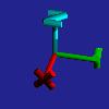
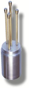
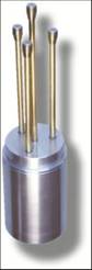
- The Soundfield microphone allows for simultaneous measurements of the
omnidirectional pressure and of the three cartesian components of
particle velocity (figure-of-8 patterns)
|
|
35
|
|
|
36
|
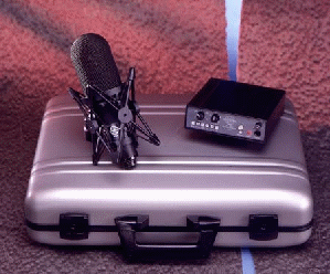
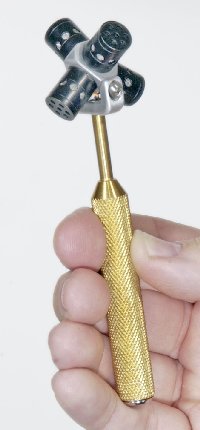
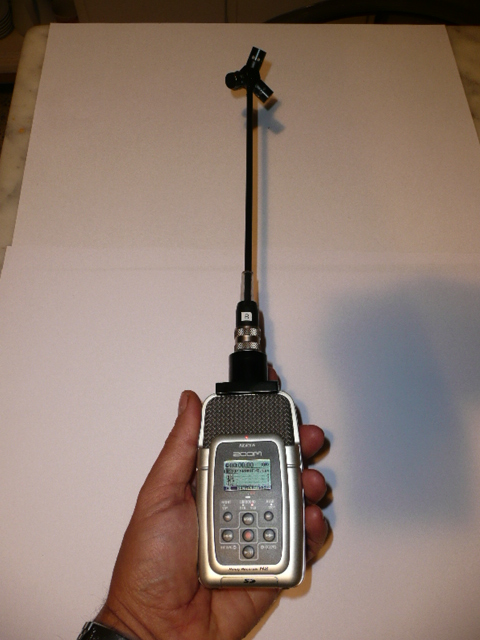
- Today several alternatives to Soundfield microphones do exists. All of
them are providing “raw” signals from the 4 capsules, and the conversion
from these signals (A-format) to the standard Ambisonic signals
(B-format) is performed digitally by means of software running on the
computer
|
|
37
|
- The original idea of Michael Gerzon was finally put in practice in 2003,
thanks to the Israeli-based company WAVES
- More than 50 theatres all around the world were measured, capturing 3D
IRs (4-channels B-format with a Soundfield microphone)
- The measurments did also include binaural impulse responses, and a
circular-array of microphone positions
- More details on WWW.ACOUSTICS.NET
|
|
38
|
|
|
39
|
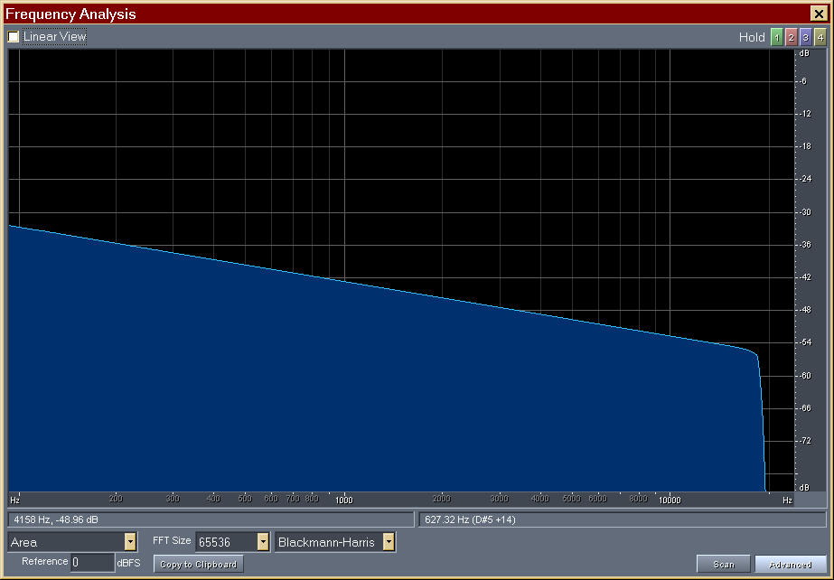
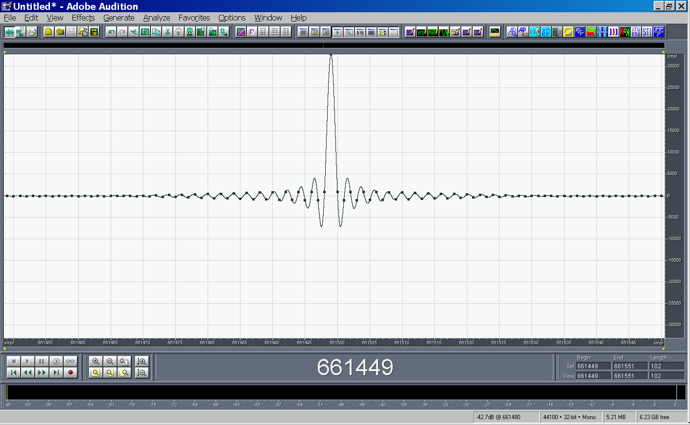
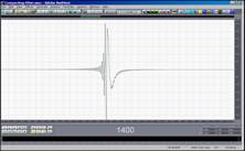
- Pre-ringing at high frequency due to improper fade-out
|
|
40
|
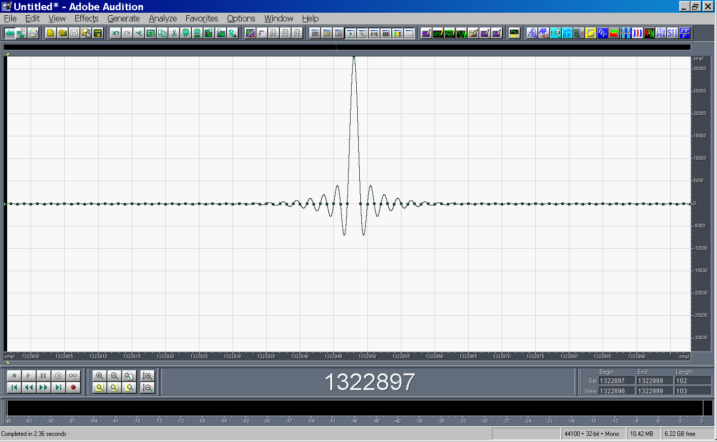
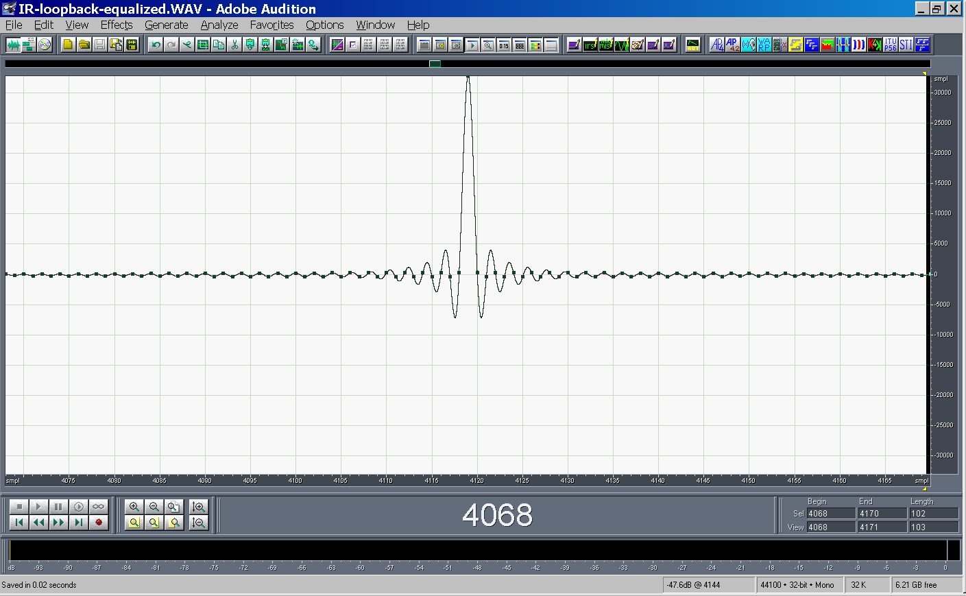
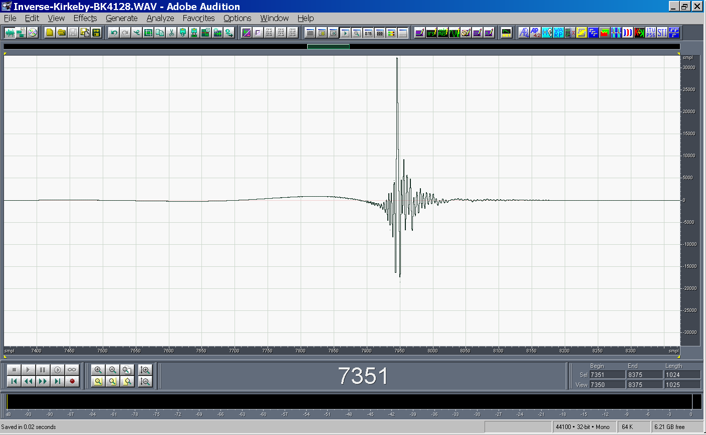
- Perfect Dirac’s delta after removing the fade-out
|
|
41
|
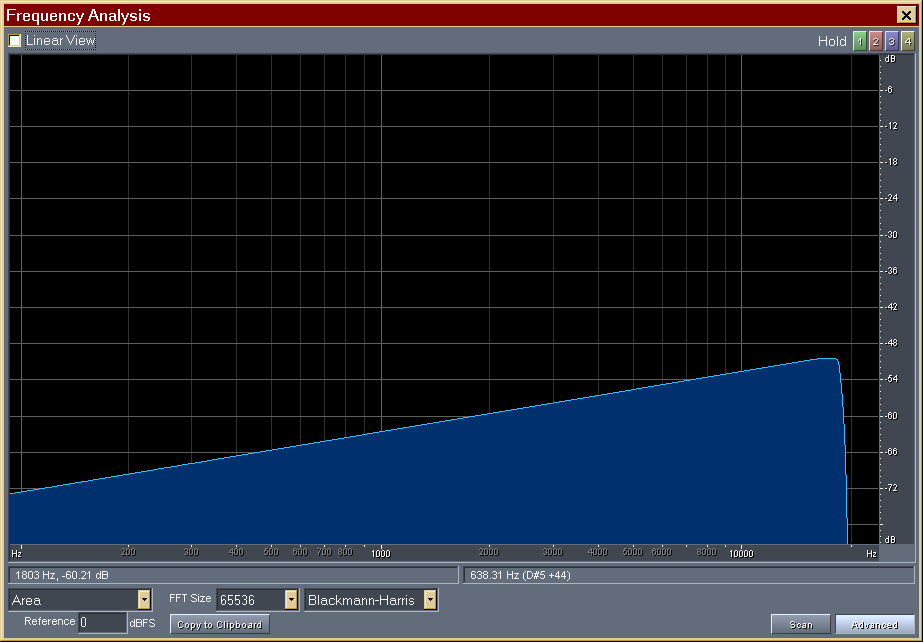
- Pre-ringing at low frequency due to a bad sound card featuring
frequency-dependent latency
|
|
42
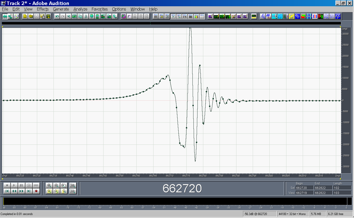
|
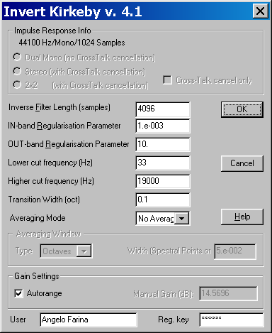
- The Kirkeby inverse filter is computed inverting the measured IR
|
|
43
|
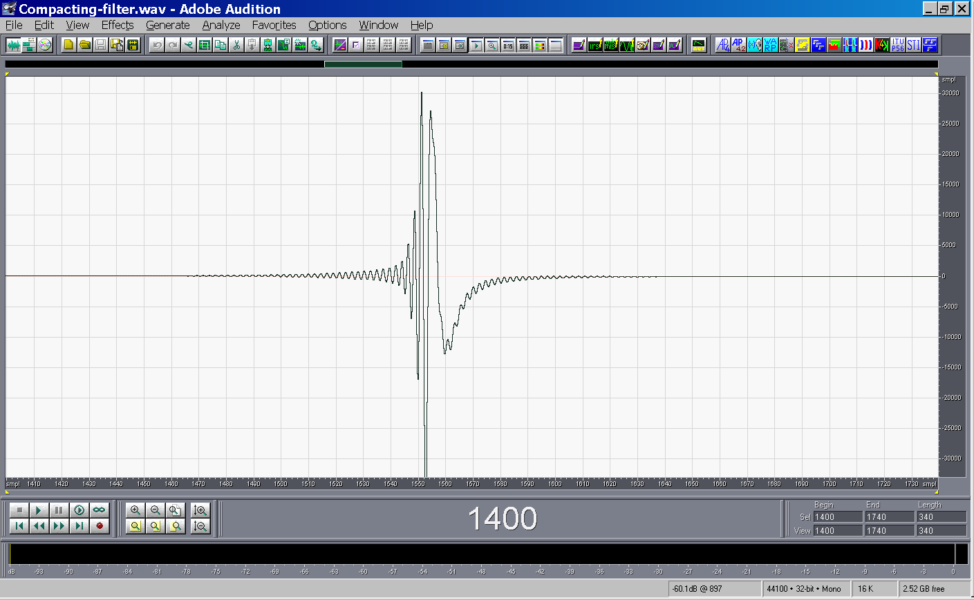
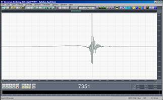
- Convolving the time-smeared IR with the Kirkeby compacting filter, a
very sharp IR is obtained
|
|
44
|
|
|
45
|
- An anechoic measurement is first performed
|
|
46
|
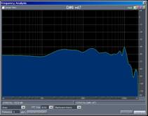
- A suitable inverse filter is generated with the Kirkeby method by
inverting the anechoic measurement
|
|
47
|
- The inverse filter can be either pre-convolved with the test signal or
post-convolved with the result of the measurement
- Pre-convolution usually reduces the SPL being generated by the
loudspeaker, resulting in worst S/N ratio
- On the other hand, post-convolution can make the background noise to
become “coloured”, and hence more perciptible
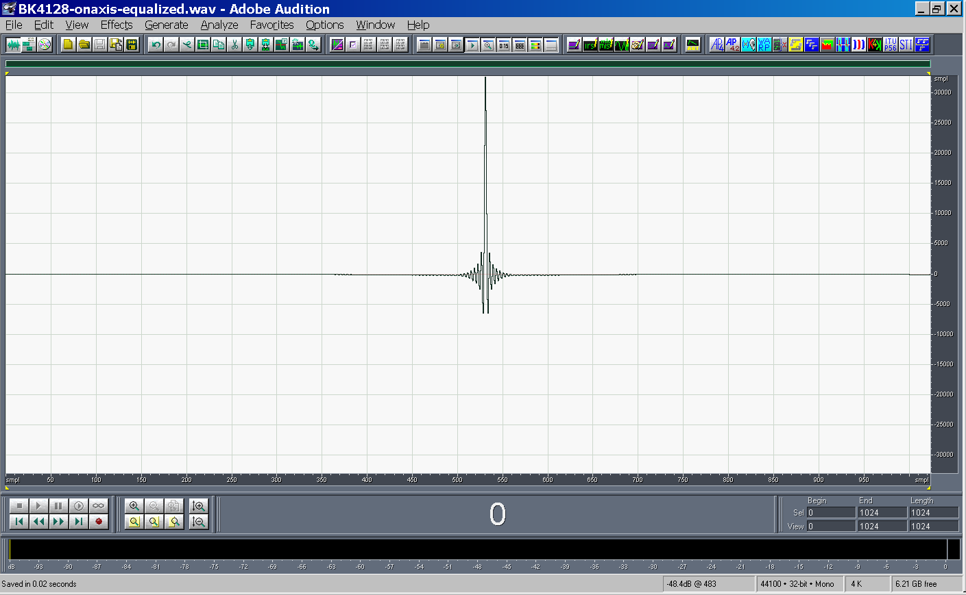
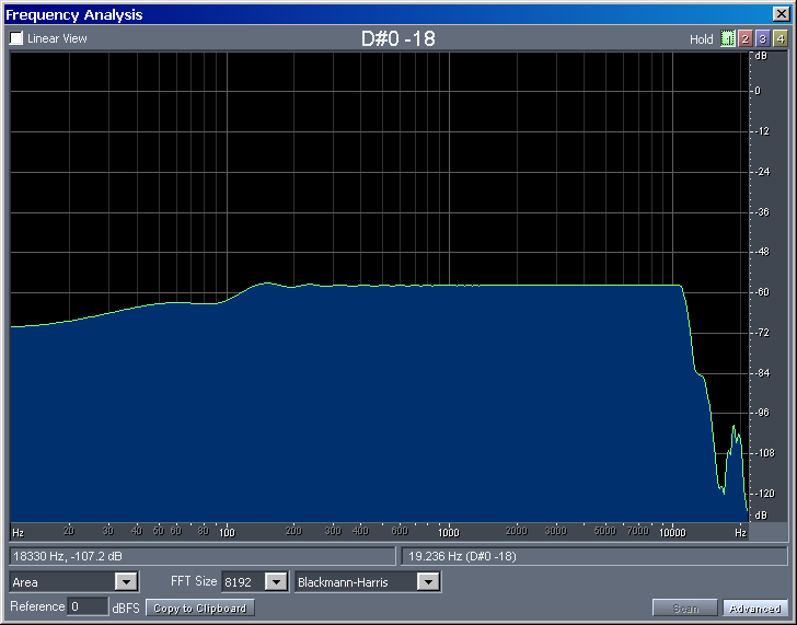
- The resulting anechoic IR becomes almost perfectly a Dirac’s Delta
function:
|
|
48
|
|
|
49
|
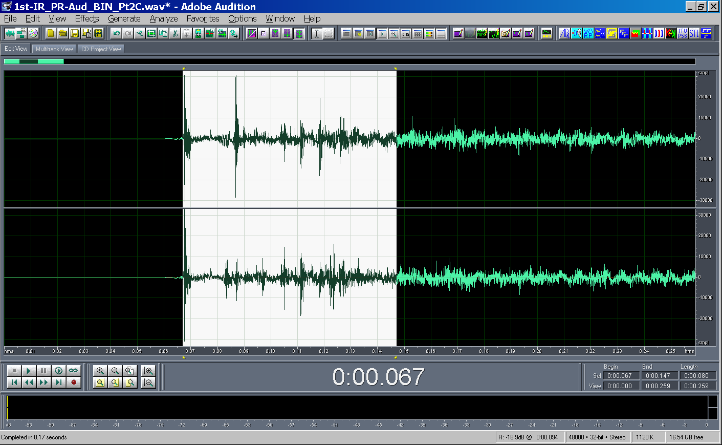
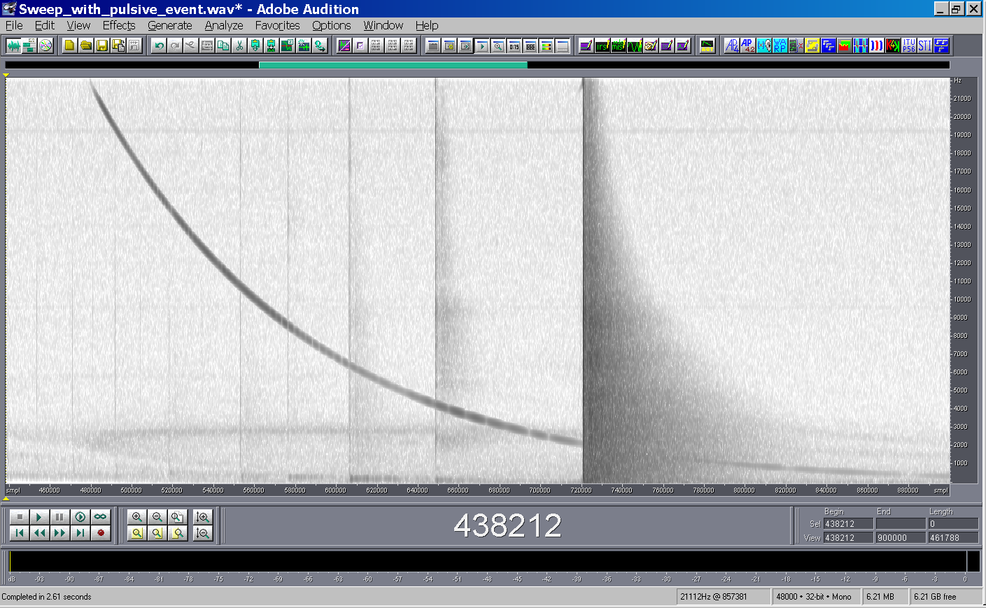
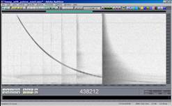
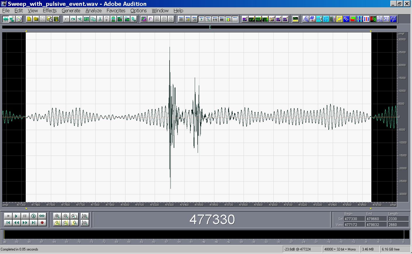
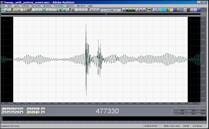
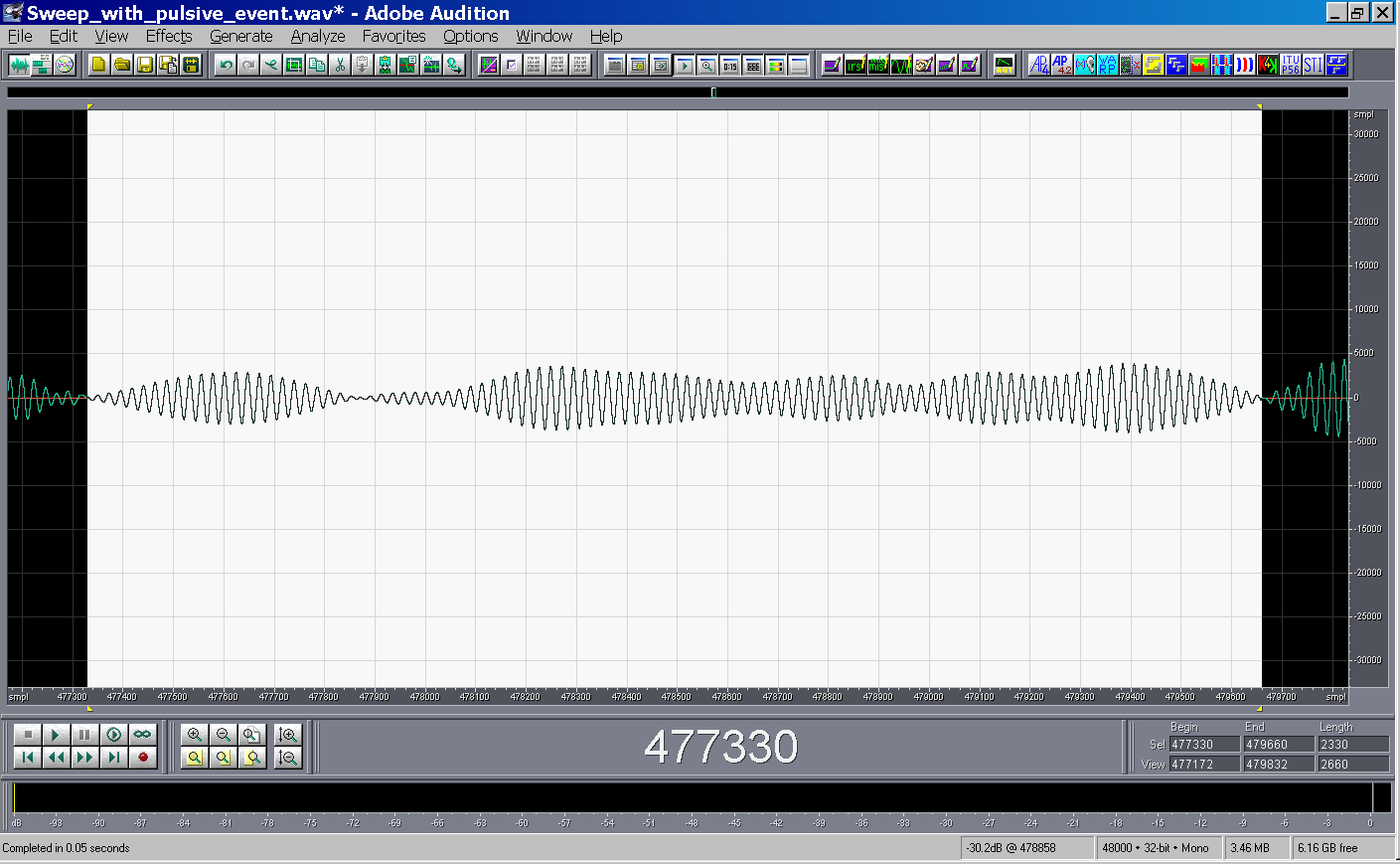
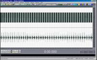
- Often a pulsive noise occurs during a sine sweep measurement
|
|
50
|
- After deconvolution, the pulsive sound causes untolerable artifacts in
the impulse response
|
|
51
|
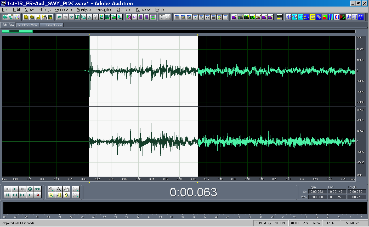
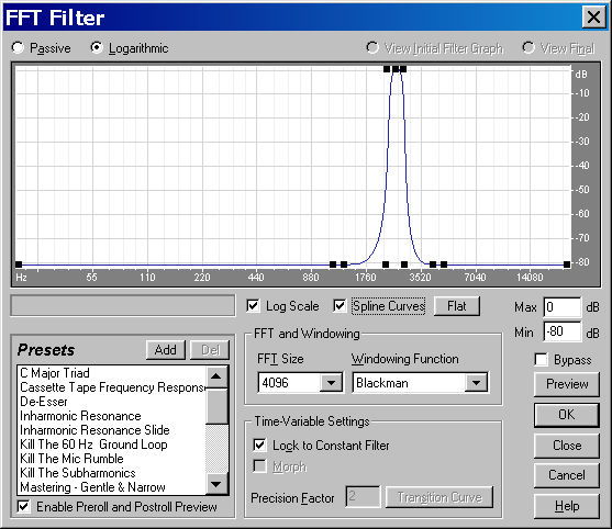
- Several denoising techniques can be employed:
- Brutely silencing the transient noise
- Employing the specific “click-pop eliminator” plugin of Adobe Audition
- Applying a narrow-passband filter around the frequency which was being
generated in the moment in which the pulsive noise occurred
- The third approach provides the better results:
|
|
52
|
|
|
53
|
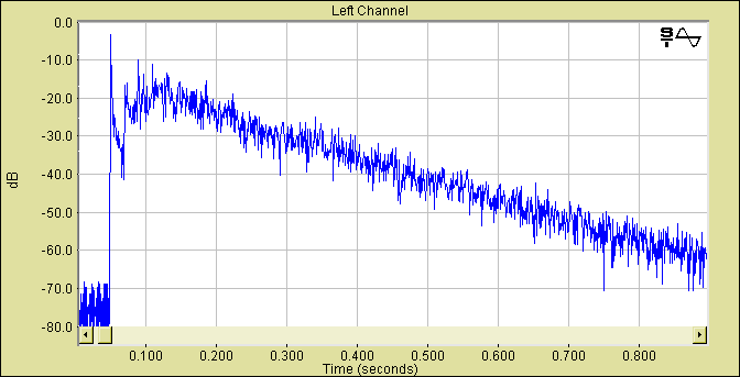
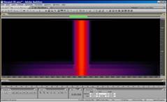
- When the measurement is performed employing devices which exhibit
signifcant clock mismatch between playback and recording, the resulting
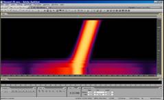
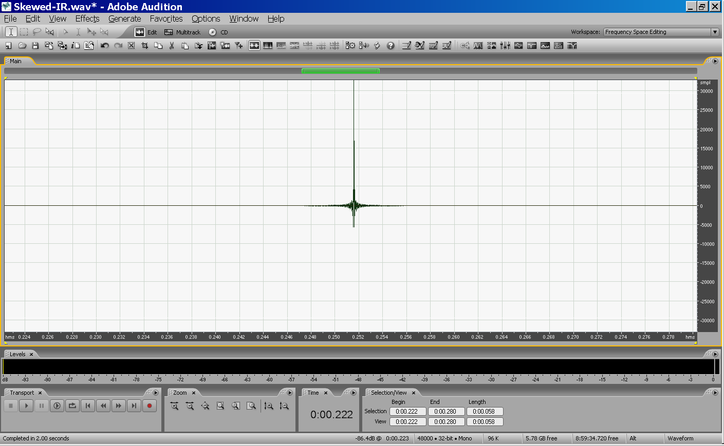
impulse response is “skewed” (stretched in time):
|
|
54
|
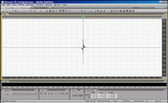
- It is possible to re-pack the impulse response employing the
already-described approach based on the usage of a Kirkeby inverse
filter:
|
|
55
|
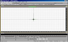
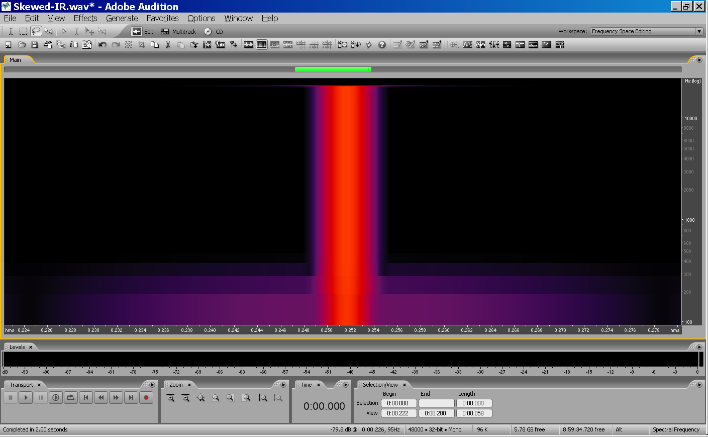
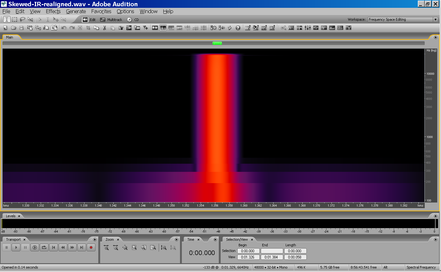
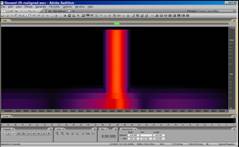
- However, it is always possible to generate a pre-stretched inverse
filter, which is longer or shorter than the “theoretical” one - by
proper selection of the lenght of the inverse filter, it is possible to
deconvolve impulse responses which are almost perfectly “unskewed”:
|
|
56
|
|
|
57
|
- When several impulse response measurements are synchronously-averaged
for improving the S/N ratio, the late part of the tail cancels out,
particularly at high frequency, due to slight time variance of the
system
|
|
58
|
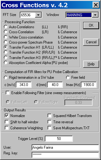
- However, if averagaing is performed properly in spectral domain, and a
single conversion to time domain is performed after averaging, this
artifact is significantly reduced
- The new “cross Functions” plugin can be used for computing H1:
|
|
59
|
|
|
60
|
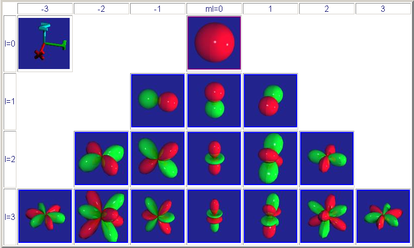
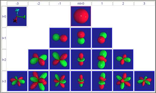
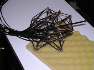
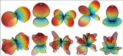
- Microphone arrays capable of synthesizing aribitrary directivity
patterns
- Advanced spatial analysis of the sound field employing spherical
harmonics (Ambisonics - 1° order or higher)
- Loudspeaker arrays capable of synthesizing arbitrary directivity
patterns
- Generalized solution in which both the directivities of the source and
of the receiver are represented as a spherical harmonics expansion
|
|
61
|
- The answer is simple: analyze the spatial distribution of both source
and receiver by means of higher-order spherical harmonics expansion
- Spherical harmonics analysis is the equivalent, in space domain, of the
Fourier analysis in time domain
- As a complex time-domain waveform can be though as the sum of a number
of sinusoidal and cosinusoidal functions, so a complex spatial
distribution around a given notional point can be expressed as the sum
of a number of spherical harmonic functions
|
|
62
|
|
|
63
|
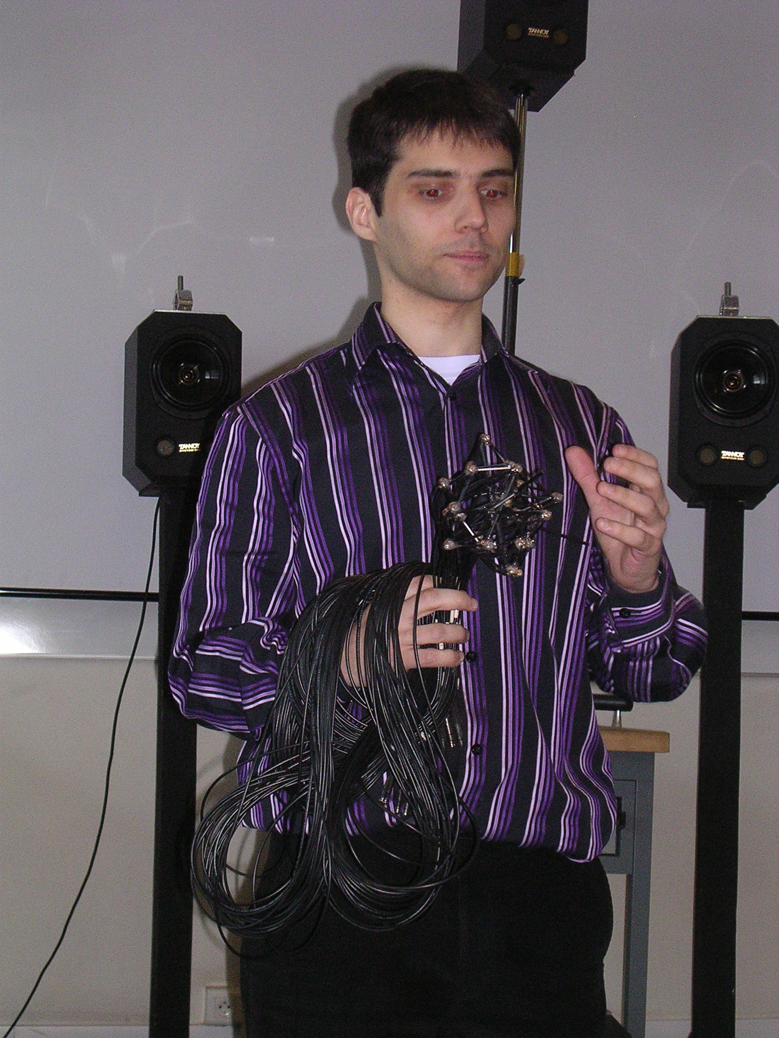
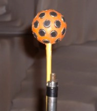
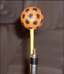
- Arnoud Laborie developed a 24-capsule compact microphone array - by
means of advanced digital filtering, spherical ahrmonic signals up to 3°
order are obtained (16 channels)
|
|
64
|
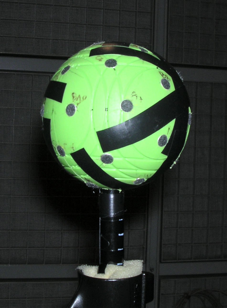
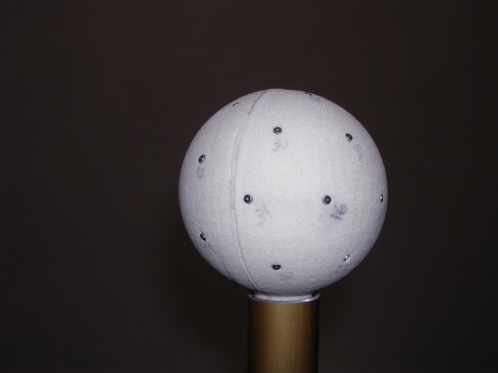
- Jerome Daniel and Sebastien Moreau built samples of 32-capsules
spherical arrays - these allow for extractions of microphone signals up
to 4° order (25 channels)
|
|
65
|
|
|
66
|
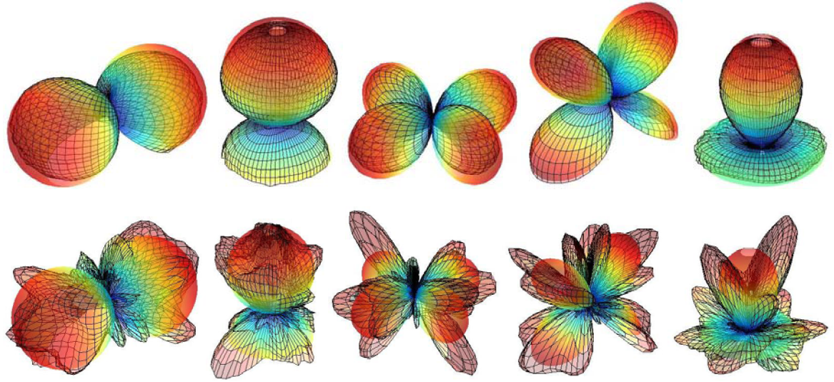
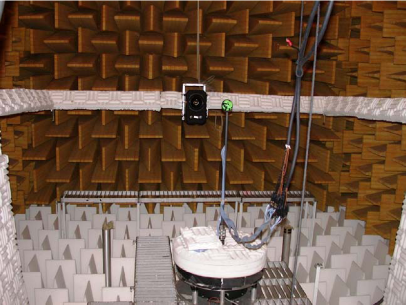
- Sebastien Moreau and Olivier Warusfel verified the directivity patterns
of the 4°-order microphone array in the anechoic room of IRCAM (Paris)
|
|
67
|
- Current 3D IR sampling is still based on the usage of an
“omnidirectional” source
- The knowledge of the 3D IR measured in this way provide no information
about the soundfield generated inside the room from a directive source
(i.e., a musical instrument, a singer, etc.)
- Dave Malham suggested to represent also the source directivity with a
set of spherical harmonics, called O-format - this is perfectly
reciprocal to the representation of the microphone directivity with the
B-format signals (Soundfield microphone).
- Consequently, a complete and reciprocal spatial transfer function can be
defined, employing a 4-channels O-format source and a 4-channels
B-format receiver:
|
|
68
|
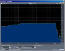
- LookLine D200 dodechaedron
|
|
69
|
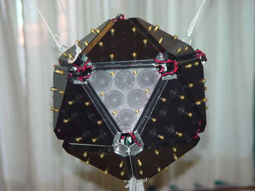
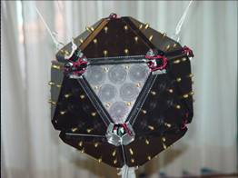
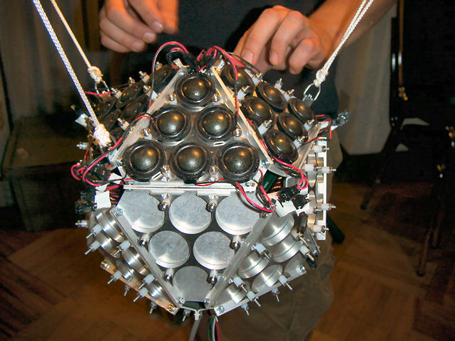
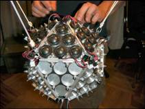
- Adrian Freed, Peter Kassakian, and David Wessel (CNMAT) developed a new
120-loudspeakers, digitally controlled sound source, capable of
synthesizing sound emission according to spherical harmonics patterns up
to 5° order.
|
|
70
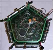
|
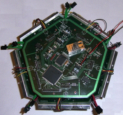
- Class-D embedded amplifiers
|
|
71
|
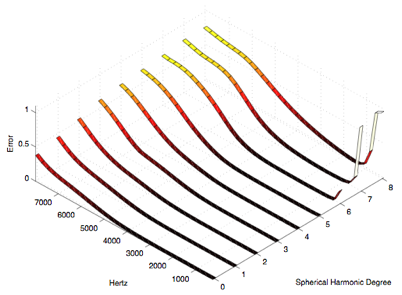
- The spatial reconstruction error of a 120-loudspeakers array is
frequency dependant, as shown here:
|
|
72
|
- Employing massive arrays of transducers, it will be feasible to sample
the acoustical temporal-spatial transfer function of a room
- Currently available hardware and software tools make this practical only
up to 4° order, which means 25 inputs and 25 outputs
- A complete measurement for a given source-receiver position pair takes
approximately 10 minutes (25 sine sweeps of 15s each are generated one
after the other, while all the microphone signals are sampled
simultaneously)
- However, it has been seen that real-world sources can be already
approximated quite well with 2°-order functions, and even the human HRTF
directivites are reasonally approximated with 3°-order functions.
|
|
73
|
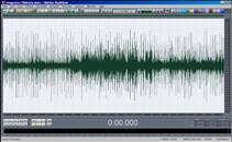
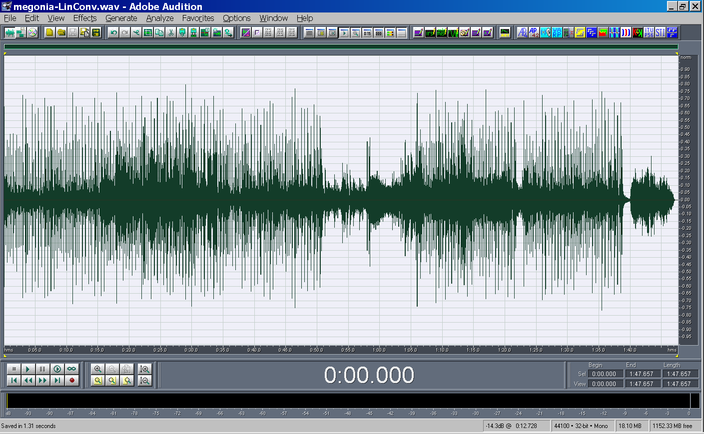
- Often impulse responses are measured for being employed in auralization
systems (i.e. Waves)
- Linear convolution is employed for this
- This method indeed does not sound realistic, as it removes any
not-linear effect
- We can now exploy the results of an ESS measurement for performing a
not-linear convolution
- For this, indeed, the measured “harmonic orders IRs” have to be
transformed into corresponding Volterra kernels
|
|
74
|
- The basic approach is to convolve separately, and then add the result,
the linear IR, the second order IR, the third order IR, and so on.
- Each order IR is convolved with the input signal raised at the
corresponding power:
|
|
75
|
- A simple linear system allows for computation of Volterra Kernels
starting from the measured “harmonic orders” IRs
|
|
76
|
- As we have got the Volterra kernels already in frequency domain, we can
efficiently use them in a multiple convolution algorithm implemented by
overlap-and-save of the partitioned input signal:
|
|
77
|
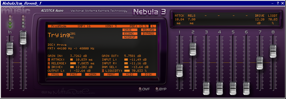
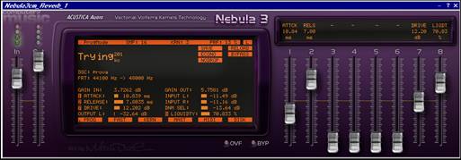
- A small Italian startup company, Acustica Audio, developed a VST plugin
based on the Diagonal Volterra Kernel method, named Nebula
|
|
78
|
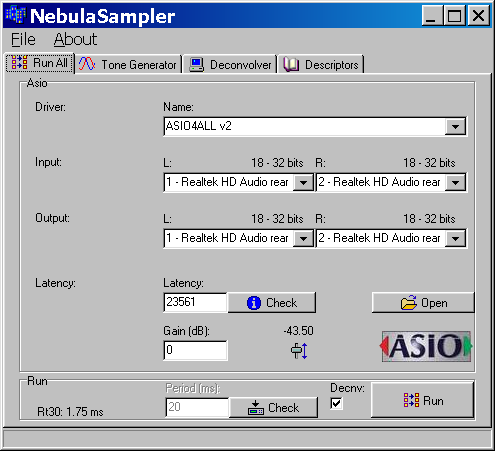
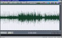
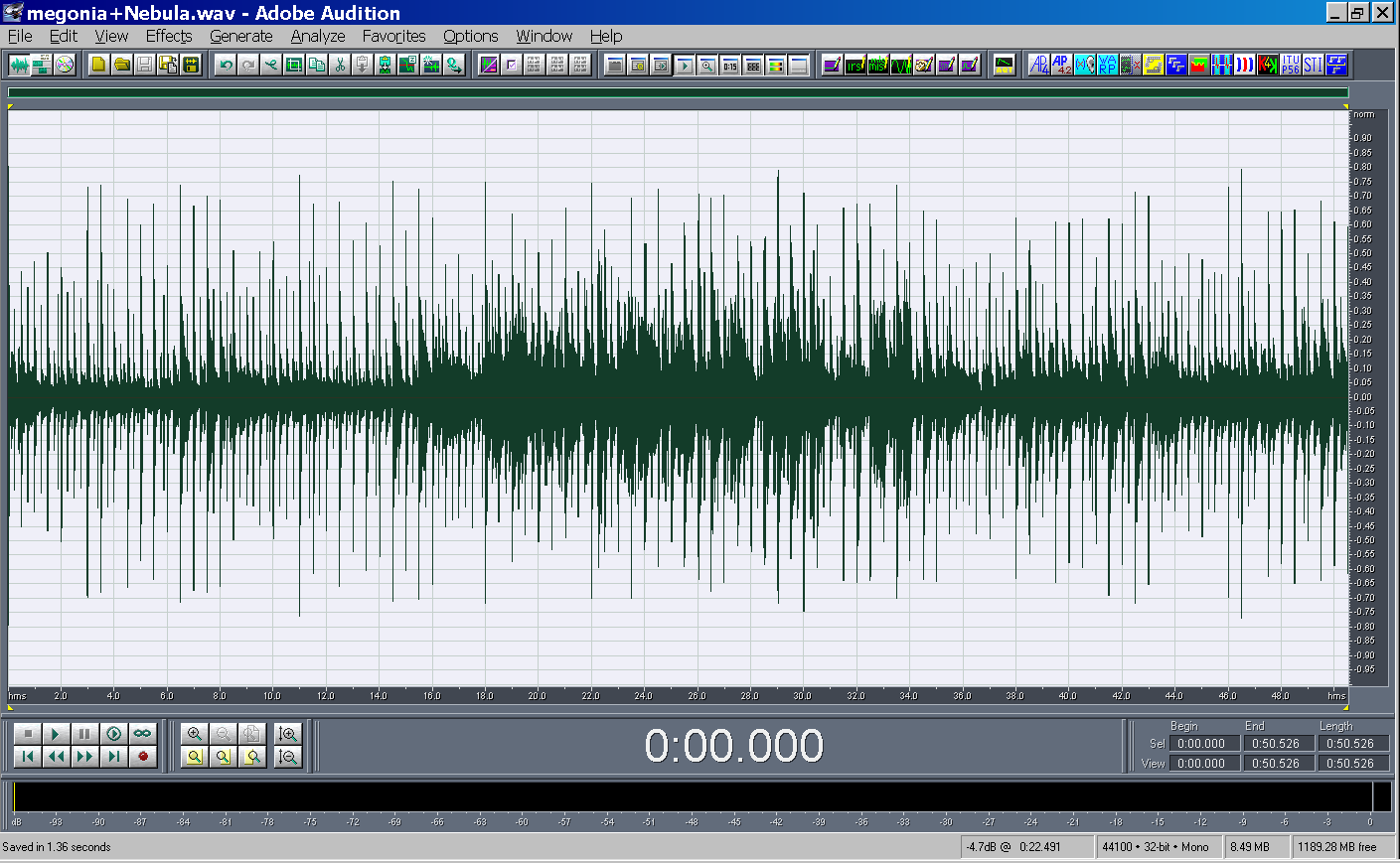
- Nebula is also equipped with a companion application, Nebula Sampler,
designed for automatizing the measurement of a not linear system with
the Exponential Sine Sweep method:
|
|
79
|
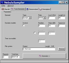
- Nebula can sample also time-variant systems, such as flangers or
compressors, by repeating the sine sweep measurement several times,
along a repetition cycle or changing the signal amplitude
|
|
80
|
- Nebula is actually limited to Volterra kernels up to 5th order, and consequently does not
emulates high-frequency harmonics:
|
|
81
|
|
|
82
|
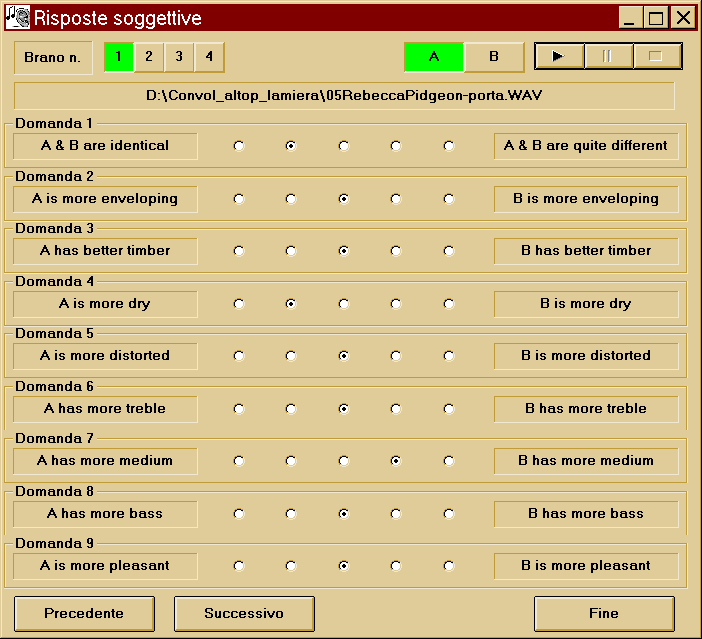
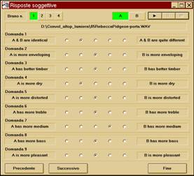
- A/B comparison
- Live recording & non-linear auralization
- 12 selected subjects
- 4 music samples
- 9 questions
- 5-dots horizontal scale
- Simple statistical analysis of the results
- A was the live recording, B was the auralization, but the listener did
not know this
|
|
83
|
- Statistical parameters – more advanced statistical methods would be
advisable for getting more significant results
|
|
84
|
|
|
85
|
- The sine sweep method revealed to be systematically superior to the MLS
& TDS methods for measuring electroacoustical impulse responses
- The ESS method also allows for measurement of not-linear devices and to
assess harmonic distortion
- Current limitation for spatial analysis in room acoustis is due to
transducers (loudspeakers and microphones)
- A new generation of loudspeakers and microphones, made of massive
arrays, is under development.
- The “harmonic orders” impulse responses obtained by the exponential sine
sweep method can be used for not-linear convolution, which yields more
realistic auralization
|

 Notes
Notes