Differentiation and Integration of Audio Signals
What's the audible effect of the well-known mathematical operations of differentiation and integration, when applied to a sound sample?
Do you want to listen at the derivative or integral of your own voice?
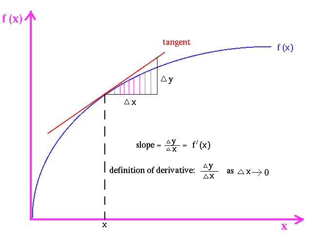
From Maths to soundMany students at high school and university do not "grasp" the real meaning of the usual operations of differentiation or integration of a function. Maths teachers tend to explain these operators by means of "graphical" concepts, such as:
"the derivative of a given function is the slope of the curve at any point"
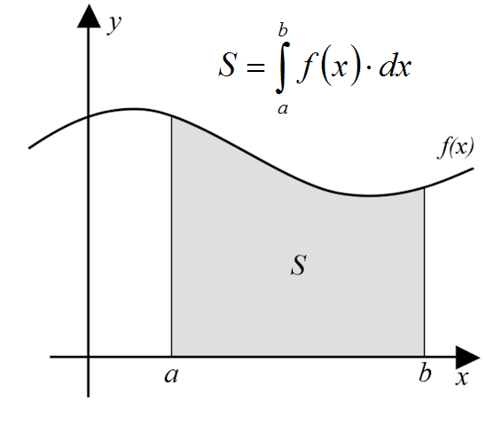
"the integral of a given function is the area subtended under the curve, between two points"
The following figures show these concepts:
 |
 |
Albeit these geometrical concepts can be useful for some specific scientific applications (for example, the analysis of historical series of the values of foreign exchanges or stock actions), they are of little value for understanding the application of the differentiation and integration operators to real-world realms, such as differentiating an image, a sound, and in general most time-varying quantities related to human perceptions, such as vibrations, temperature, air speed, etc.
Here we present the effect of the differentiation and integration operators applied to a sound signal. In particular, we start from a PCM (Pulse Code Modulation) digitally-sampled waveform of the human voice. This is obtained by first converting the sound pressure in an electric voltage signal, by means of a condenser microphone. Then the electrical waveform is sampled by means of an Analog-to-Digital converter, at a sampling rate of 48 kHz (that is, 48000 samples per seconds are collected). Each sample is a floating-point number, bounded in the range +/- 1.
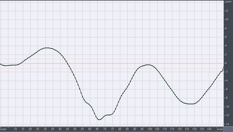
The following figure shows a very short piece of such a digitally-sampled waveform:
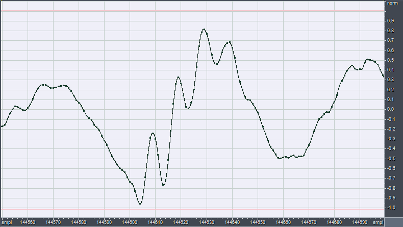
So the sound is nothing else than a very long sequence of floating-point numbers. As the time interval Dt between two adjacent samples is very small (1/48000 s), we can compute the derivative of our waveform following its definition, that is, taking the difference between the value of each sample and the value of the preceding sample:
x'(t) = x(t) - x(t-1)
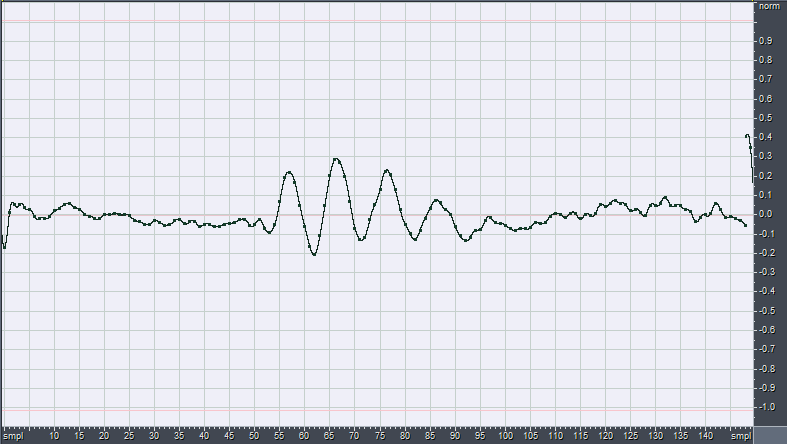
If we do that to the waveform of the preceding example, we get the following new waveform x':
Similarly, for computing the "running" integral between zero-time and the current time, we can simply sum the values of all the preceding samples:
y(t) = x(t) + x(t-1) + x(t-2) + .... + x(0)
Applying this computation to the original waveform, we get the following integrated waveform y:
It must be noted how the amplitude of the integrated waveform is now much larger than the original, and it exceeds the "full scale boundaries" of +/-1. For rebounding it inside the full-scale limits, it becomes necessary to reduce the gain by approximately 22 dB.
Looking at the waveforms, it can be seen that the integrated one is very smooth and round, whilst the differentiated one is very spiky and rough. This means that the integrated one contains a lot of energy at low frequency (waveforms with long period), whilst the differentiated one contains more energy at high frequency (waveform with very short period).
Mathematically, this can be explained if we assume that our waveform is obtained as the sum of a number of sinusoidal signals with proper amplitudes and phases (Fourier theorem):
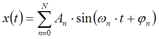
When dealing with audio signals, it must be said that, in general, the conditions of validity of the Fourier theorem are NOT met. So the Fourier analysis of a real waveform provides a misleading representation of reality. Nevertheless, we ca still learn something useful employing the Fourier approach, albeit we must keep in mind that some artifacts can occur.
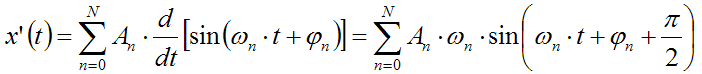
As both differentiation and integral, when applied to a sum of functions, can be applied directly to each of the addends, we get:
Differentiation:
Integral:
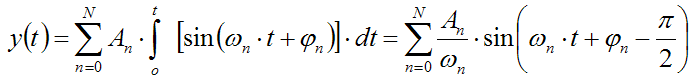
This means that the differentiated signals will have spectral components with amplitude increasing linearly with frequency. Instead, the integrated signal will have spectral components with amplitude decreasing proportionally with frequency. In practice, the spectrum of the signal is being tilted, and the slope of the spectrum is increased by 6dB/octave in case of differentiation and reduced by 6dB/octave in case of integration.
The following figure shows how the spectrum of a "white noise" is altered by the two mathematical operators (a "white noise" is a signal having flat spectrum, that is, composed by sinusoids all having the same amplitude An):
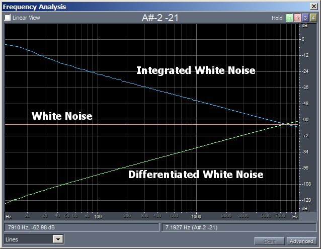
Note that the three spectra cross at 8000 Hz, that is, exactly 1/6 of the sampling frequency.
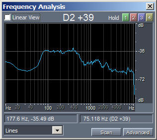
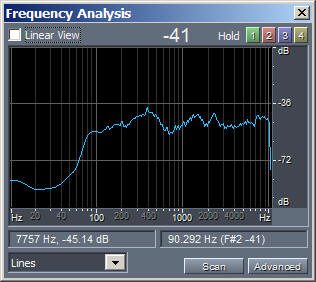
Now that we know how to compute the differentiation and integral of a sampled audio waveform, we can try to apply this process to a sample of human voice. The following figures, with linked MP3 audible sound samples, show this:
 |
 |
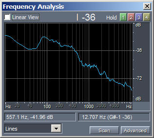 |
| Original.mp3 | Differentiated.mp3 | Integrated.mp3 |
Please note that the amplitude of processed waveforms was rescaled, for making them easily audible without having to change the volume during playback.
Now we try to re-frame all the previous knowledge within the scheme of LTI (Linear, Time Invariant) filters. Many effects applied to a sound can be framed in such a scheme: delays, echoes, reverb, spectral equalization, basic filtering such as low-pass, high-pass, band-pass and band-reject, shelf-filtering, etc.
However, not all audio effects can be represented as a linear, time-invariant filter: for example this scheme does not applies to compressors, automatic gain control, soft-clipping, gating, flanging, time-varying delay (Doppler effect), saturation, harmonic enhancement, etc.
Luckily, differentiation and integration are LTI filters. So we can represented them thanks to the convolution theorem, employing an impulse response of finite length h(t) (that is, employing FIR filtering):
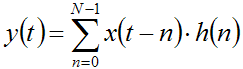
This formula is usually read as "y is the convolution of x with h". The operation "sum of products" is called convolution, and is a very trivial operation indeed.
This is usually written in short form as
|
y(t) = x(t) * h(t) |
where the operator * is called the convolution operator.
The length N of the impulse response h is not critical for the differentiation operator. Instead, for the integral operator, in theory an infinite length would be needed. Truncating the length of the corresponding FIR filter to a given value imposes a low-frequency limit, that is, the computed integral signal will be correct only above a frequency given by the reciprocal of the length of the FIR filter itself.
For example, if we choose a filter length N = 4800 samples (0.1s), we get a correct filtering above 10 Hz, which is plenty enough for audio applications.
So what is the time-domain representation (waveform) of such FIR filters, for performing differentiation and integration?
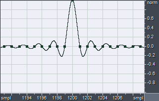
We start defining the Dirac's Delta function d(t) filter: it is a "null" filter, which does not alter the processed waveform at all.
The Dirac's Delta function is simply a waveform containing a zero amplitude for all samples, except for one sample which has a value of +1.0:
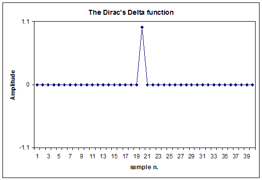
If a signal is convolved with d(t), the result is identical to the original signal (no filtering), except for a delay due to the position of the not-zero value inside the Dirac's Delta FIR filter (20 samples in the example above). It must also be said that the spectrum if a Dirac's Delta function is perfectly flat (white).
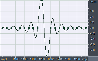
If we now differentiate the Dirac's Delta function, we get what is known as the Unit Doublet function u1(t) (click here for a mathematical definition of this functions).
In practice, the difference between zeroes remain zero, and this occurs for all the samples of the differentiated signals, except for two consecutive ones, which will get respectively the values of +1.0 and -1.0, as shown here:

This Unit Doublet function u1(t) is in practice a differentiating FIR filter: if an x(t) signal is convolved with u1(t), the result will be the time-derivative of the original signal:

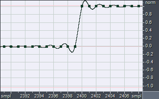
If we instead apply the integration operator to the Dirac's Delta function, we obtain the Unit Step function, also called Heaviside step function H(t):
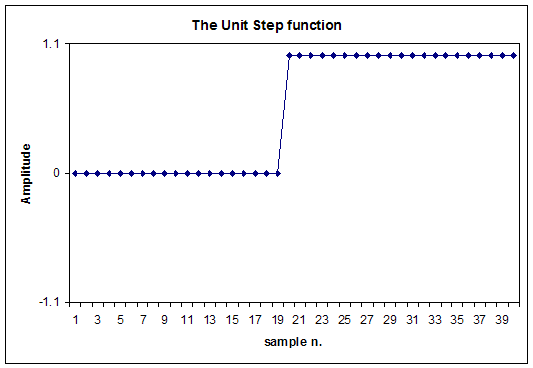
As already said, in this case we should continue the integration for a long time, ensuring to get a FIR filter of enough length, for obtaining proper integration over all the audio spectrum (down to less than 16 Hz, the minimum audible frequency).
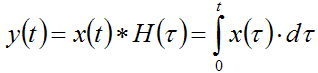
This Unit Step function H(t) is in practice an integrating FIR filter: if an x(t) signal is convolved with H(t), the result will be the time-integral of the original signal:
 |
 |
 |
| Dirac.wav | Derivator-Filter.wav | Integrator-Filter.wav |
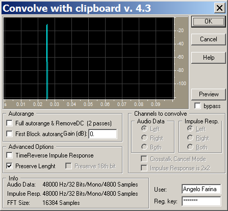
You can use these FIR filters with any software capable of performing linear convolution, for example Matlab, or Adobe Audition, or Audacity; for the latter two, the Aurora Plugins can be used, which contain a very handy-to-use "convolve with clipboard" module:
A very useful exercise is first to apply differentiation, followed by integration (or vice-versa): as differentiation is the opposite of integration, the two operations elide each other, reconstructing the original signal. And, of course, if the two FIR filters are convolved each other, the Dirac's Delta function is obtained as the result:
d(t) = u1(t) * H(t)
Finally, it must be said that second-order differentiation or integration can be easily obtained by repeating twice the convolution of the signal with the corresponding filter.
Last point is: when the hell one has the need to differentiate or integrate an audio signal? In reality, this often occurs when "strange" types of transducers have been used: for example, an accelerometer, so the sampled signal is an acceleration, and the user wants to transform it into velocity (simple integration) or displacement (double integration). And, of course, the opposite is also possible: if one has sampled the position of a vibrating surface (for example by means of a laser distance meter), and wants to obtain velocity or acceleration, then he has to differentiate the recorded signal once or twice...
So this article describes a general method for processing audio signals (or, indeed, any sampled waveform), for performing differentiation and integration numerically, and very efficiently (convolution is amazingly fast when properly implemented as "partitioned convolution" on modern processors).